An Exploration of Machine Learning Methods for Robust Boredom Classification Using EEG and GSR Data


Abstract
1. Introduction
2. Background
3. Data Collection Methodology
3.1. Participants
3.2. Sensors
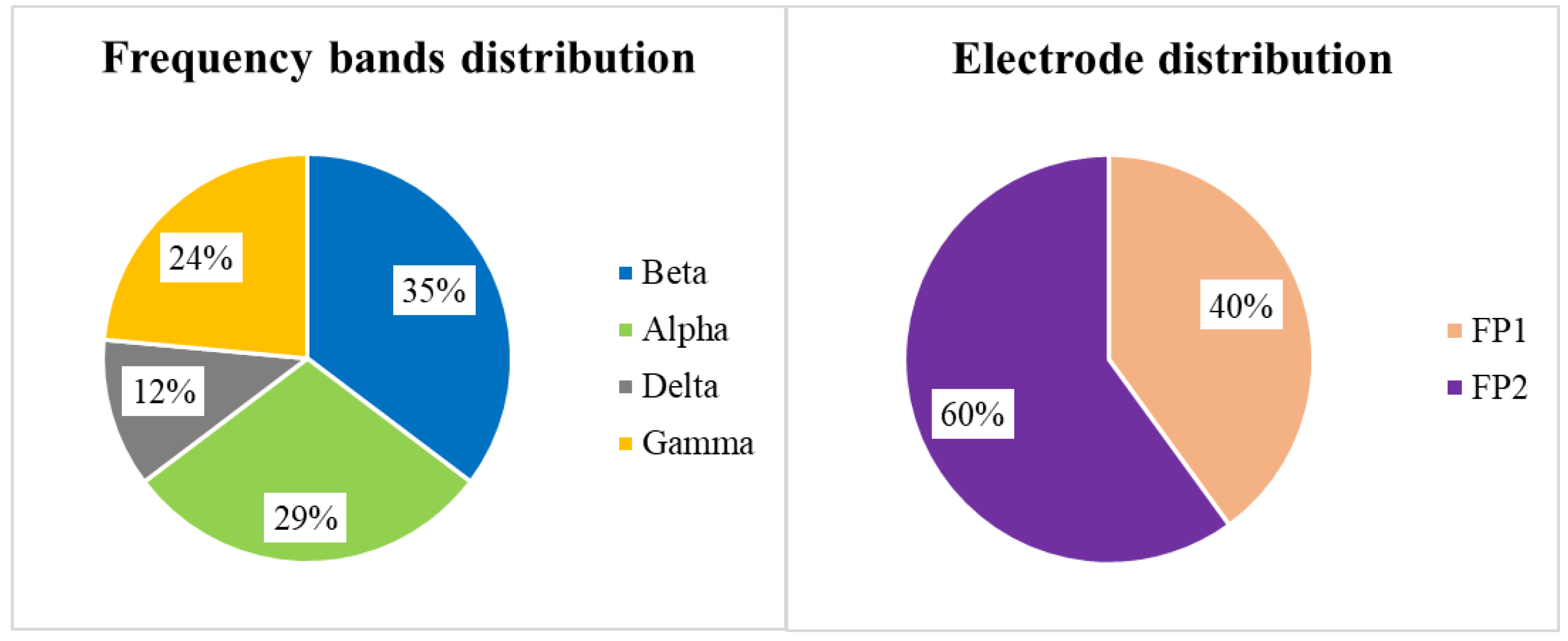
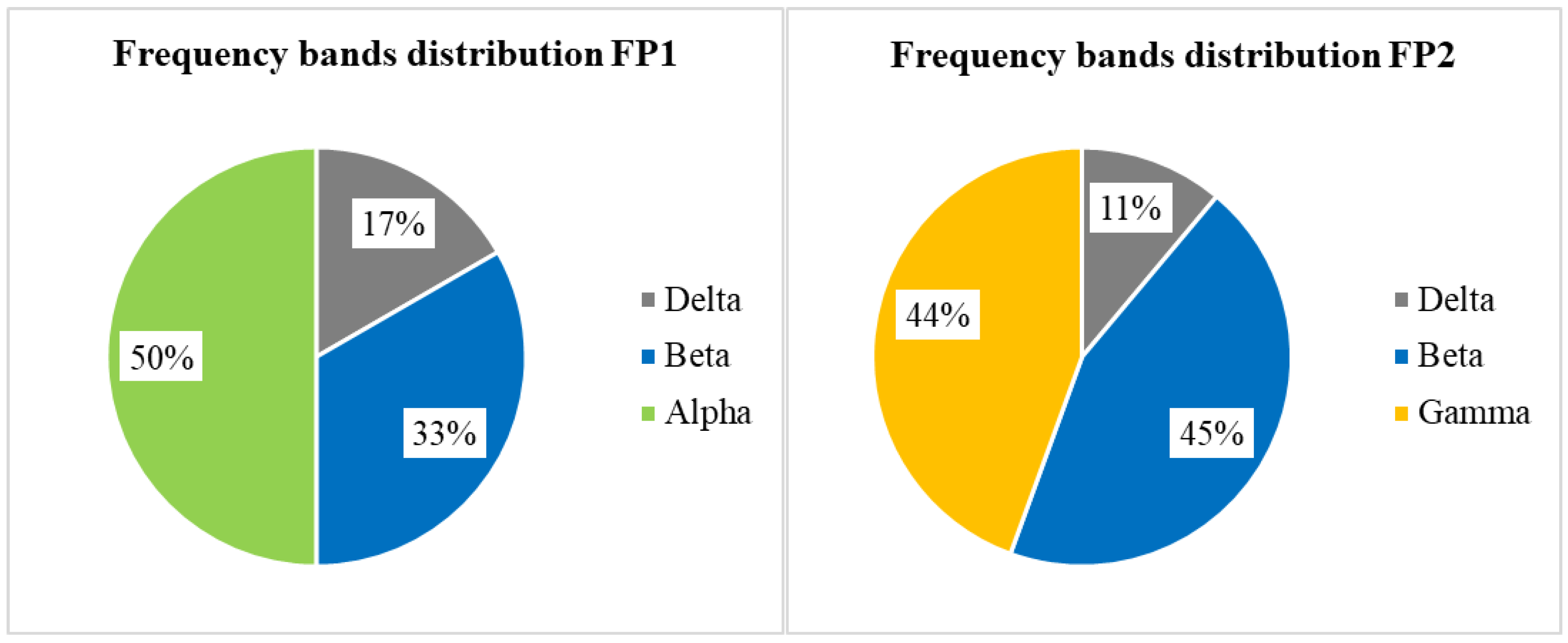
- Delta: (1–4) Hz,
- Theta: (4–8) Hz,
- Alpha: (7.5–13) Hz,
- Beta: (13–30) Hz,
- Gamma: (30–44) Hz.
3.3. Protocol
4. Machine Learning Methods
4.1. Window Size
4.2. Features
4.2.1. EEG
4.2.2. GSR
4.3. Machine Learning Model Selection
4.4. Feature Refinement
5. Results
5.1. Questionnaire
5.2. Initial Test for Model Selection
5.3. Hyperparameter Tuning
5.3.1. Random Forest
- Number of features to randomly investigate: 1–6, default = int(),
- Number of trees: 1–100,
- Maximum depth of trees: 1–50, no limit.
5.3.2. Multilayer Perceptron
- Learning rate: 0.01–1.00 (0.01 unit),
- Epoch: 1–2000 (1 unit).
5.3.3. Naïve Bayes
5.4. Final Performance Analysis
5.4.1. Performance Measurement
5.4.2. Analysis of the Selected Features
6. Discussion
7. Conclusions
Author Contributions
Funding
Acknowledgments
Conflicts of Interest
References
- Picard, R.W. Affective Computing; MIT Press: Cambridge, MA, USA, 1995; pp. 1–16. [Google Scholar]
- Shen, L.; Wang, M.; Shen, R. Affective e-Learning: Using “Emotional” Data to Improve Learning in Pervasive Learning Environment Related Work and the Pervasive e-Learning Platform. Educ. Technol. Soc. 2009, 12, 176–189. [Google Scholar]
- Zheng, W.L.; Lu, B.L. Investigating Critical Frequency Bands and Channels for EEG-Based Emotion Recognition with Deep Neural Networks. IEEE Trans. Auton. Mental Dev. 2015, 7, 162–175. [Google Scholar] [CrossRef]
- Zheng, W.L.; Zhu, J.Y.; Lu, B.L. Identifying Stable Patterns over Time for Emotion Recognition from EEG. IEEE Trans. Affect. Comput. 2017, 417–429. [Google Scholar] [CrossRef]
- Kim, J.J.; Fesenmaier, D.R. Measuring emotions in real time: Implications for tourism experience design. J. Travel Res. 2015, 54, 419–429. [Google Scholar] [CrossRef]
- Kim, J.; Seo, J.; Laine, T.H. Detecting Boredom from Eye Gaze and EEG. Biomed. Signal Process. Control 2018, 46, 302–313. [Google Scholar] [CrossRef]
- Seo, J.; Laine, T.H.; Sohn, K.A. Machine learning approaches for boredom classification using eeg. J. Ambient Intell. Human. Comput. 2019, 10, 3831–3846. [Google Scholar] [CrossRef]
- Giakoumis, D.; Vogiannou, A.; Kosunen, I.; Moustakas, K.; Tzovaras, D.; Hassapis, G. Identifying Psychophysiological Correlates of Boredom and Negative Mood Induced During HCI. In Proceedings of the 1st International Workshop on Bio-Inspired Human-Machine Interfaces and Healthcare Applications, Valencia, Spain, 21 January 2010; pp. 3–12, ISBN 9789896740207. [Google Scholar]
- Giakoumis, D.; Tzovaras, D.; Moustakas, K.; Hassapis, F. Automatic recognition of boredom in video games using novel biosignal moment-based features. IEEE Trans. Affect. Comput. 2011, 2, 119–133. [Google Scholar] [CrossRef]
- Jang, E.H.; Park, B.J.; Park, M.S.; Kim, S.H.; Sohn, J.H. Analysis of physiological signals for recognition of boredom, pain, and surprise emotions. J. Physiol. Anthropol. 2015, 34, 1–12. [Google Scholar] [CrossRef]
- Mandryk, R.L.; Atkins, M.S. A fuzzy physiological approach for continuously modeling emotion during interaction with play technologies. Int. J. Hum. Comput. Stud. 2007, 65, 329–347. [Google Scholar] [CrossRef]
- Sidney, K.D.; Craig, S.D.; Gholson, B.; Franklin, S.; Picard, R.; Graesser, A.C. Integrating Affect Sensors in an Intelligent Tutoring System. In Proceedings of the Affective Interactions: The Computer in the Affective Loop Workshop at 2005 International Conference on Intelligent User Interfaces, San Diego, CA, USA, 10–13 January 2005; pp. 7–13. [Google Scholar]
- Jaques, N.; Conati, C.; Harley, J.M.; Azevedo, R. Predicting affect from gaze data during interaction with an intelligent tutoring system. In Lecture Notes in Computer Science; 8474 LNCS; Springer: Berlin, Germany, 2014; pp. 29–38. [Google Scholar]
- Thompson, W.T.; Lopez, N.; Hickey, P.; DaLuz, C.; Caldwell, J.L.; Tvaryanas, A.P. Effects of Shift Work and Sustained Operations: Operator Performance in Remotely Piloted Aircraft (Op-Repair); Technical report; 311th Human Systems Wing Brooks Air Force Base: San Antonio, TX, USA, 2006. [Google Scholar]
- Britton, A.; Shipley, M.J. Bored to death? Int. J. Epidemiol. 2010, 39, 370–371. [Google Scholar] [CrossRef]
- Kanevsky, L.S. A comparative study of children’s learning in the zone of proximal development. Eur. J. High Ab. 1994, 5, 163–175. [Google Scholar] [CrossRef]
- Oroujlou, N.; Vahedi, M. Motivation, attitude, and language learning. Proc. Soc. Behav. Sci. 2011, 29, 994–1000. [Google Scholar] [CrossRef]
- Sottilare, R.; Goldberg, B. Designing adaptive computer-based tutoring systems to accelerate learning and facilitate retention. J. Cogn. Technol 2012, 17, 19–33. [Google Scholar]
- Yeager, D.S.; Henderson, M.D.; Paunesku, D.; Walton, G.M.; D’Mello, S.; Spitzer, B.J.; Duckworth, A.L. Boring but important: A self-transcendent purpose for learning fosters academic self-regulation. J. Personal. Soc. Psychol. 2014, 107, 5592014. [Google Scholar] [CrossRef] [PubMed]
- Baker, R.; D’Mello, S.; Rodrigo, M.; Graesser, A. Better to be frustrated than bored: The incidence and persistence of affect during interactions with three different computer-based learning environments. Int. J. Hum. Comput. Stud. 2010, 68, 223–241. [Google Scholar] [CrossRef]
- Fagerberg, P.; Ståhl, A.; Höök, K. EMoto: Emotionally engaging interaction. Pers. Ubiquitous Comput. 2004, 8, 377–381. [Google Scholar] [CrossRef]
- Feldman, L. Variations in the circumplex structure of mood. Personal. Soc. Psychol. Bull. 1995, 21, 806–817. [Google Scholar] [CrossRef]
- Li, M.; Lu, B.-L. Emotion classification based on gamma-band EEG. In Proceedings of the 2009 Annual International Conference of the IEEE Engineering in Medicine and Biology Society, Minneapolis, MN, USA, 3–6 September 2009; pp. 1223–1226. [Google Scholar]
- Lin, Y.P.; Wang, C.H.; Jung, T.P.; Wu, T.L.; Jeng, S.K.; Duann, J.R.; Chen, J.H. EEG-based emotion recognition in music listening. IEEE Trans. Biomed. Eng. 2010, 57, 1798–1806. [Google Scholar]
- Shen, L.; Leon, E.; Callaghan, V.; Shen, R. Exploratory research on an Affective e-Learning Model. In Proceedings of the Workshop on Blended Learning, Edinburgh, UK, 15–17 August 2007; pp. 267–278, ISBN 978-3-540-78138-7. [Google Scholar]
- Russell, J.A. A circumplex model of affect. J. Personal. Soc. Psychol. 1980, 39, 1161–1178. [Google Scholar] [CrossRef]
- Vogel-Walcutt, J.J.; Fiorella, L.; Carper, T.; Schatz, S. The definition, assessment, and mitigation of state boredom within educational settings: A comprehensive review. Educ. Psychol. Rev. 2012, 24, 89–111. [Google Scholar] [CrossRef]
- Eastwood, J.D.; Frischen, A.; Fenske, M.J.; Smilek, D. The Unengaged Mind: Defining Boredom in Terms of Attention. Perspect. Psycholog. Sci. 2012, 7, 482–495. [Google Scholar] [CrossRef] [PubMed]
- Fahlman, S.A.; Mercer-Lynn, K.B.; Flora, D.B.; Eastwood, J.D. Development and Validation of the Multidimensional State Boredom Scale. Assessment 2013, 20, 68–85. [Google Scholar] [CrossRef] [PubMed]
- Sanei, S.; Chambers, J.A. EEG Signal Processing; John Wiley & Sons: Hoboken, NJ, USA, 2013; ISBN 978-0-470-02581-9. [Google Scholar]
- Ashwal, S.; Rust, R. Child neurology in the 20th century. Pediatr. Res. 2003, 53, 345. [Google Scholar] [CrossRef] [PubMed]
- Martini, F.H.; Bartholomew, E.F. Essentials of Anatomy and Physiology; Benjamin Cummings: San Francisco, CA, USA, 2002; ISBN 978-0-13-061567-1. [Google Scholar]
- Carlson, N.R. Physiology of Behavior; Allyn & Bacon: Boston, MA, USA, 2012; ISBN 978-0-205-23939-9. [Google Scholar]
- Bench, S.W.; Lench, H.C. On the function of boredom. Behav. Sci. 2013, 3, 459–472. [Google Scholar] [CrossRef]
- World Medical Association. World Medical Association Declaration of Helsinki. Ethical principles for medical research involving human subjects. Bull. World Health Organ. 2001, 79, 373–374. [Google Scholar]
- MUSE. MUSE TM Headband. Available online: http://www.choosemuse.com/ (accessed on 19 October 2019).
- Seeed. Grove—GSR Sensor. Available online: http://wiki.seeedstudio.com/Grove-GSR{_}Sensor/ (accessed on 19 October 2019).
- Jasper, H. Report of the committee on methods of clinical examination in electroencephalography: 1957. Electroencephalogr. Clin. Neurophysiol. 1958, 10, 370–375. [Google Scholar]
- Lang, P.J.; Bradley, M.M.; Cuthbert, B.N. International Affective Picture System (IAPS): Affective Ratings of Pictures and Instruction Manual; Technical Report A-8; University of Florida: Gainesville, FL, USA, 2008. [Google Scholar]
- Hall, M.; Frank, E.; Holmes, G.; Pfahringer, B.; Reutemann, P.; Witten, I.H. The WEKA data mining software: An update. ACM SIGKDD Explor. Newsl. 2009, 11, 10–18. [Google Scholar] [CrossRef]
- Kohavi, R.; John, G.H. Wrappers for feature subset selection. Artif. Intell. 1997, 97, 273–324. [Google Scholar] [CrossRef]
- Muller, M.P.; Tomlinson, G.; Marrie, T.J.; Tang, P.; McGeer, A.; Low, D.E.; Detsky, A.S.; Gold, W.L. Can Routine Laboratory Tests Discriminate between Severe Acute Respiratory Syndrome and Other Causes of Community-Acquired Pneumonia? Clin. Infect. Dis. 2005, 40, 1079–1086. [Google Scholar] [CrossRef]


| Study | Data Source | Number of Participants |
|---|---|---|
| Shen et al. [2] | HR, GSR, BP, EEG | 1 |
| Mandryk and Atkins [11] | HR, GSR, Facial | 12 |
| Kim et al. [6] | Eye-tracking, EEG | 16 |
| Giakoumis et al. [9] | ECG, GSR | 19 |
| Giakoumis et al. [8] | ECG, GSR | 21 |
| Seo et al. [7] | EEG | 28 |
| D’Mello et al. [12] | Facial, Gesture | 30 |
| Jaques et al. [13] | Eye-tracking | 67 |
| Jang et al. [10] | HR, GSR, Temperature, PPG | 217 |
| Study | Accuracy | Method |
|---|---|---|
| Jaques et al. [13] | 73.0% | Random Forest |
| Jang et al. [10] | 84.7% | Discriminant Function Analysis |
| Shen et al. [2] | 86.3% | Support Vector Machine (SVM) |
| Seo et al. [7] | 86.7% | k-Nearest Neighbors (kNN) |
| Giakoumis et al. [9] | 94.2% | Linear Discriminant Analysis |
| Mandryk and Atkins [11], D’Mello et al. [12], Giakoumis et al. [8], and Kim et al. [6] | Not available | Statistical approaches |
| Algorithm | Option | Algorithm | Option | Algorithm | Option |
|---|---|---|---|---|---|
| IBk | Default | Multilayer Perceptron (MLP) | t | SVM | Linear |
| 1/distance | i | Polynomial | |||
| 1-distance | a | Radial | |||
| Decision Stump | Default | o | Sigmoid | ||
| Decision Table | Default | t,a | LMT | Default | |
| Hoeffding Tree | Default | t,a,o | PART | Default | |
| J48 | Default | t,i,a,o | Logistic | Default | |
| Random Tree (RT) | Default | Random Forest (RF) | Default | Simple Logistic | Default |
| JRip | Default | REP Tree | Default | Zero R | Default |
| Naïve Bayes (NB) | Default | KStar | Default | One R | Default |
| EEG-GSR | EEG | GSR | |||
|---|---|---|---|---|---|
| Algorithm | Accuracy (%) | Algorithm | Accuracy (%) | Algorithm | Accuracy (%) |
| RF | 83.93 | RF | 80.36 | MLP (t) | 75.00 |
| PART | 80.36 | MLP (a) | 78.57 | Simple Logistic | 73.21 |
| IBk | 80.36 | MLP (i) | 78.57 | MLP (a) | 71.43 |
| J48 | 80.36 | KStar | 78.57 | MLP (i) | 71.43 |
| NB | 80.36 | MLP (o) | 73.21 | SVM (Radial Kernel) | 71.43 |
| RT | 78.57 | NB | 71.43 | MLP (o) | 69.64 |
| Hoeffding Tree | 78.57 | Hoeffding Tree | 71.43 | KStar | 69.64 |
| MLP (o) | 76.79 | MLP (t) | 71.43 | PART | 69.64 |
| MLP (a) | 76.79 | IBk | 71.43 | Decision Stump | 69.64 |
| MLP (t) | 76.79 | Logistic | 69.64 | J48 | 69.64 |
| Features | Trees | Depth | Accuracy (%) | AUC | |
|---|---|---|---|---|---|
| EEG-GSR | default (7) | 14 | 7 | 87.50 | 0.842 |
| 2 | 14 | 7 | 87.50 | 0.842 | |
| 3 | 14 | 7 | 87.50 | 0.842 | |
| EEG | default (6) | 18 | no limit | 76.79 | 0.780 |
| default (6) | 18 | 11 | 76.79 | 0.780 | |
| default (6) | 18 | 12 | 76.79 | 0.780 | |
| GSR | default (3) | 18 | no limit | 76.79 | 0.780 |
| default (3) | 18 | 11 | 76.79 | 0.780 | |
| default (3) | 18 | 12 | 76.79 | 0.780 |
| Layer and Node | Learning Rate | Epoch | Accuracy (%) | AUC | |
|---|---|---|---|---|---|
| EEG-GSR | a | 0.47 | 444 | 76.79 | 0.771 |
| i | 0.90 | 215 | 82.14 | 0.794 | |
| o | 0.47 | 444 | 76.79 | 0.771 | |
| t | 0.76 | 73 | 83.93 | 0.765 | |
| i, a | 0.59 | 572 | 82.14 | 0.795 | |
| i, o | 0.49 | 1351 | 82.14 | 0.764 | |
| t, i | 0.91 | 192 | 76.79 | 0.737 | |
| EEG | a | 0.70 | 452 | 76.79 | 0.733 |
| i | 0.19 | 489 | 83.93 | 0.822 | |
| o | 0.21 | 654 | 80.36 | 0.751 | |
| t | 0.48 | 163 | 82.14 | 0.791 | |
| i, a | 0.43 | 405 | 78.57 | 0.706 | |
| i, o | 0.71 | 265 | 75.00 | 0.710 | |
| t, i | 0.99 | 320 | 78.57 | 0.692 | |
| GSR | a | 0.44 | 312 | 75.00 | 0.767 |
| i | 0.44 | 312 | 75.00 | 0.767 | |
| o | 0.44 | 312 | 75.00 | 0.767 | |
| t | 0.95 | 321 | 76.79 | 0.759 | |
| i, a | 0.64 | 1120 | 73.21 | 0.663 | |
| i, o | 0.90 | 231 | 71.43 | 0.642 | |
| t, i | 0.91 | 255 | 71.43 | 0.641 |
| Kernel | Discretization | Accuracy (%) | AUC | |
|---|---|---|---|---|
| EEG-GSR | FALSE | FALSE | 82.14 | 0.785 |
| TRUE | FALSE | 76.79 | 0.819 | |
| FALSE | TRUE | 60.71 | 0.569 | |
| EEG | FALSE | FALSE | 67.86 | 0.653 |
| TRUE | FALSE | 67.86 | 0.603 | |
| FALSE | TRUE | 53.57 | 0.454 | |
| GSR | FALSE | FALSE | 69.64 | 0.681 |
| TRUE | FALSE | 64.29 | 0.626 | |
| FALSE | TRUE | 60.71 | 0.569 |
| Accuracy (%) | AUC | Time (ms) | ||||||
|---|---|---|---|---|---|---|---|---|
| Mean | Max | Min | Mean | Max | Min | Mean | ||
| EEG-GSR | RF | 77.53 | 89.29 | 66.07 | 0.815 | 0.900 | 0.722 | 26.52 |
| NB | 79.39 | 85.71 | 67.86 | 0.783 | 0.819 | 0.733 | 9.41 | |
| MLP | 79.98 | 83.93 | 71.43 | 0.781 | 0.815 | 0.723 | 70.98 | |
| EEG | RF | 64.77 | 78.57 | 51.79 | 0.695 | 0.833 | 0.569 | 44.38 |
| NB | 70.85 | 78.57 | 64.29 | 0.710 | 0.760 | 0.640 | 9.89 | |
| MLP | 77.04 | 83.93 | 66.07 | 0.775 | 0.833 | 0.641 | 251.22 | |
| GSR | RF | 68.33 | 78.57 | 53.57 | 0.731 | 0.831 | 0.591 | 30.84 |
| NB | 66.86 | 71.43 | 64.29 | 0.709 | 0.751 | 0.655 | 11.9 | |
| MLP | 70.03 | 76.79 | 60.71 | 0.744 | 0.796 | 0.683 | 163.49 | |
| EEG-GSR | EEG | GSR | |
|---|---|---|---|
| MLP | ABP Delta FP1 std | ABP Beta FP2 mean | MV std NMV mean |
| ABP Gamma FP2 mean | ABP Gamma FP2 mean | ||
| NABP Delta FP2 mean | NABP Alpha FP1 std | ||
| MV std | DASM Alpha | ||
| NB | ABP Beta FP2 mean | NABP Alpha FP1 std DE Beta FP1 | MV std NMV std |
| ABP Gamma FP2 mean | |||
| NABP Alpha FP1 mean | |||
| NABP Beta FP1 mean | |||
| MV std | |||
| RF | NABP Beta FP2 mean MV std | ABP Gamma FP2 mean | MV std SR mean |
| NABP Beta FP2 mean | |||
| Alpha RASM |
© 2019 by the authors. Licensee MDPI, Basel, Switzerland. This article is an open access article distributed under the terms and conditions of the Creative Commons Attribution (CC BY) license (http://creativecommons.org/licenses/by/4.0/).
Share and Cite
Seo, J.; Laine, T.H.; Sohn, K.-A. An Exploration of Machine Learning Methods for Robust Boredom Classification Using EEG and GSR Data. Sensors 2019, 19, 4561. https://doi.org/10.3390/s19204561
Seo J, Laine TH, Sohn K-A. An Exploration of Machine Learning Methods for Robust Boredom Classification Using EEG and GSR Data. Sensors. 2019; 19(20):4561. https://doi.org/10.3390/s19204561
Chicago/Turabian StyleSeo, Jungryul, Teemu H. Laine, and Kyung-Ah Sohn. 2019. "An Exploration of Machine Learning Methods for Robust Boredom Classification Using EEG and GSR Data" Sensors 19, no. 20: 4561. https://doi.org/10.3390/s19204561
APA StyleSeo, J., Laine, T. H., & Sohn, K.-A. (2019). An Exploration of Machine Learning Methods for Robust Boredom Classification Using EEG and GSR Data. Sensors, 19(20), 4561. https://doi.org/10.3390/s19204561