Robust and Accurate Hand–Eye Calibration Method Based on Schur Matric Decomposition

Abstract

To improve the accuracy and robustness of hand–eye calibration, a hand–eye calibration method based on Schur matric decomposition is proposed in this paper. The accuracy of these methods strongly depends on the quality of observation data. Therefore, preprocessing observation data is essential. As with traditional two-step hand–eye calibration methods, we first solve the rotation parameters and then the translation vector can be immediately determined. A general solution was obtained from one observation through Schur matric decomposition and then the degrees of freedom were decreased from three to two. Observation data preprocessing is one of the basic unresolved problems with hand–eye calibration methods. A discriminant equation to delete outliers was deduced based on Schur matric decomposition. Finally, the basic problem of observation data preprocessing was solved using outlier detection, which significantly improved robustness. The proposed method was validated by both simulations and experiments. The results show that the prediction error of rotation and translation was 0.06 arcmin and 1.01 mm respectively, and the proposed method performed much better in outlier detection. A minimal configuration for the unique solution was proven from a new perspective.

1. Introduction

The combination of vision sensors and robots is a milestone in robotic intelligence, increasing the extent and efficacy of robot applications [1,2,3,4,5]. Hand–eye calibration is an important technique for bridging the transformation between a robot gripper and a robot vision sensor [6]. Its application is mainly reflected in the robot’s hand–eye coordination, guiding the robot gripper to accurately target and reach into a specified location using the machine vision system. From height work to surgery, the more sophisticated the operation, the better robot hand–eye coordination required.

Many researchers have studied hand–eye calibration, and all current methods can be divided into two categories: linear methods and iterative methods.

Linear methods are efficient and suitable for online hand–eye calibration. Shiu and Ahmad first introduced the dynamic equation AX = XB into hand–eye calibration and provided minimal configuration for a unique solution [6]. Tsai and Lens proposed a high-efficiency linear method for the equation AX = XB [7]. Chou and Kamel expressed rotation matrices using quaternions and obtained an analytical solution using Singular Value Decomposition (SVD) [8]. Lu and Chou used an eight-dimension vector to express rotation and translation and obtained a least squares solution [9]. Chen analyzed the relationship between screw movement and hand–eye calibration, and then proved that the movement of the robot gripper and vision sensor must satisfy certain geometric constraints [10]. Daniilidis solved rotation and translation simultaneously by means of a dual quaternion [11]. Park introduced canonical coordinates into the hand–eye calibration equation, which simplified the parameters [12]. Shah constructed a closed-form solution and derived the minimal configuration of the unique solution based on Kronecker product [13]. Compared with Daniilidis [11], Shah’s method was more reliable and accurate. Iterative methods are mainly used to improve the accuracy and robustness. Other authors [14,15] took the F norm of the rotation error and translation error as the cost function, and then optimized it using nonlinear methods. Horaud expressed rotation matrices using quaternions and simultaneously optimized the transformation between the robot-world and hand and eye [16]. Strobl and Hirzinger proposed a new adaptive error model that helped improve the solution to AX = XB and AX = ZB [17]. Ruland proposed a self-calibration method that took projection error as its cost function and optimized it using branch-and-bound [18].

The accuracies of the above methods strongly depend on the quality of the observation data. Therefore, preprocessing observation data is essential. Observation data preprocessing is rarely reported. Schmidt et al. [19] proposed a preprocessing method based on vector quantization, which improved the quality of observation data to a certain extent but could not identity outliers. The complexity increased from O(N) to O(N⁴), which considerably decreased the method’s efficiency.

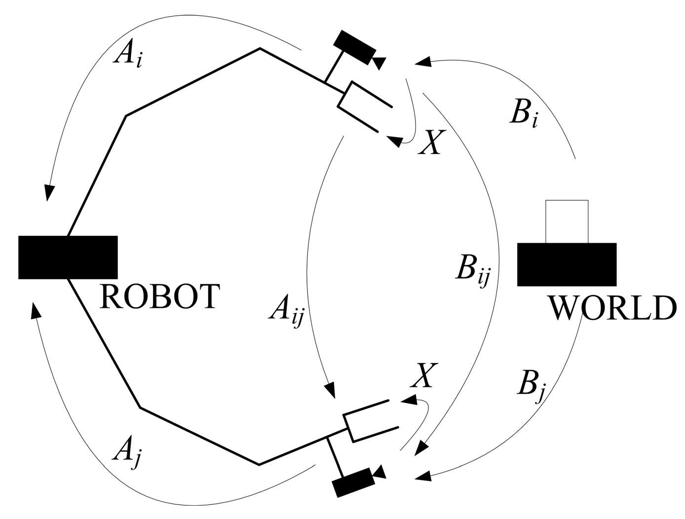
2. Description of Hand–Eye Calibration Problem

Figure 1 describes the hand–eye calibration problem. The symbols are notated as follows: G_i is the robot gripper coordinate system, it is fixed on the robot gripper and moves together with it, C_i is the camera coordinate system fixed on the camera that moves together with it and the origin point is coincident with the camera’s optical center. The Z-axis is parallel to the optical axis, and the X and Y axes are parallel to the X and Y axes of the image coordinate system. CW is the world coordinate system and RW is the robot coordinate system that is fixed on the robot and moves together with it. When the robot gripper moves, its controlling device can identify the gripper’s pose in RW.

A_i is the homogenous transformation matric from G_i to RW, obtained from the robot controlling device:

$$A_i=\left[\begin{array}{cc}{R}_{A_i}& t_{A_i}\\ 0_{1\times 3}& 1\end{array}\right]$$

(1)

B_i is the homogenous transformation matric from CW to C_i, obtained using camera pose estimation methods:

$$B_i=\left[\begin{array}{cc}{R}_{B_i}& t_{B_i}\\ 0_{1\times 3}& 1\end{array}\right]$$

(2)

A_ij is the homogenous transformation matric from G_i to G_j:

$$A_{ij}=A_j^{-1}{A}_i=\left[\begin{array}{cc}{R}_{A_{ij}}& t_{A_{ij}}\\ 0_{1\times 3}& 1\end{array}\right]$$

(3)

B_ij is the homogenous transformation matric from C_i to C_j:

$$B_{ij}=B_j{B}_i^{-1}=\left[\begin{array}{cc}{R}_{B_{ij}}& t_{B_{ij}}\\ 0_{1\times 3}& 1\end{array}\right]$$

(4)

and X is the homogenous transformation matric from C_i to G_i:

$$X=\left[\begin{array}{cc}{R}_X& t_X\\ 0_{1\times 3}& 1\end{array}\right]$$

(5)

i and j represent the ith and jth state of the robot gripper and camera respectively, ranging from 0 to N. N is the number of movements. Since the robot gripper and camera are fixed, X is constant.

The hand–eye calibration equation can be represented by notations:

$$A_{ij}X=X{B}_{ij}$$

(6)

Two equations can be obtained based on the partition matric:

$$\{\begin{array}{l}{R}_{A_{ij}}{R}_X=R_X{R}_{B_{ij}}\\ \left(R_{A_{ij}}-I\right)t_X=R_X{t}_{B_{ij}}-t_{A_{ij}}\end{array}$$

(7)

Equation (7) shows that R_X is independent, but the accuracy of t_X is related to R_X.

3. Hand–Eye Calibration Method

3.1. Schur Matric Decomposition

A given matric can be simplified to a normalized form via similarity transformation. Considering numerical stability, the similarity transformation of a unitary matric is the most attractive. Schur matric decomposition can be simply described as: If A ∈ C^n×n, then a unitary matric that satisfies U^HAU = T = D + N exists, where D is a diagonal matric and N is a strictly upper triangular matric, implicating ∀I ≥ j n_{i j} = 0. For a real matric A, U is restricted to an orthogonal matric: U^TAU = T. T has the following form:

$$T=\left[\begin{array}{cccc}{T}_{11}& T_{12}& \cdots & T_{1m}\\ 0& T_{22}& \cdots & T_{2m}\\ ⋮& ⋮& \ddots & ⋮\\ 0& 0& \cdots & T_{mm}\end{array}\right]$$

(8)

T_ii is a 1 × 1 or 2 × 2 matric consisting of complex conjugate eigenvalues. If $R_{A_{ij}}$ is similar to $R_{B_{ij}}$ and eigenvalues of $R_{A_{ij}}$ and $R_{B_{ij}}$ are the same, the matric T related to $R_{A_{ij}}$ and $R_{B_{ij}}$ are the same.

3.2. Hand–Eye Calibration Principle

A₀, B₀ is notated as the initial state of the robot gripper and camera. $\left(A_{i0},{{\rm B}}_{i0}\right)\left(i=1,2,\dots ,N-1,N\right)$ is a series of homogenous transformation matrices related to their initial states. Without the loss of generality, e.g., i = 1, only consider the equation related to the rotation in Equation (7):

$$R_{A_{10}}{R}_X=R_X{R}_{B_{10}}$$

(9)

From Theorem 1, proved in the Appendix A, the general solution can be written as:

$$R_X=U_{R_{A_{10}}}Y{U}_{R_{B_{10}}}^T$$

(10)

And

$$Y=\left[\begin{array}{ccc}\pm 1& 0& 0\\ 0& c& d\\ 0& -d& c\end{array}\right],c^2+d^2=1$$

(11)

R_X only depends on c and d. For arbitrary i = 1, 2, …, N – 1, N:

$$R_{A_{i0}}{R}_X=R_X{R}_{B_{i0}}$$

(12)

Substitute Equation (10) into Equation (12):

$$P_{i}Y=Y{Q}_i$$

(13)

where:

$$P_i=U_{R_{A_{10}}}^T{R}_{A_{i0}}{U}_{R_{A_{10}}},Q_i=U_{R_{B_{10}}}^T{R}_{B_{i0}}{U}_{R_{B_{10}}}$$

(14)

Collate Equation (13) into equations only related to s = (c d)^T.

$$C_{i}s=D_i$$

(15)

C_i is a matric generated by the coefficients of c and d. D_i is a matric generated by the constant term. Then, the final linear equation system can be constructed:

$$Cs=D$$

(16)

where,

$$C=\left[\begin{array}{c}{C}_1\\ C_2\\ ⋮\\ C_N\end{array}\right],D=\left[\begin{array}{c}{D}_1\\ D_2\\ ⋮\\ D_N\end{array}\right]$$

(17)

This is a least squares problem with constraints:

$$\begin{array}{l}s=\arg \min \left\{s^{T}Ks-2F^{T}s\right\}\\ s^{T}s=1\end{array}$$

(18)

where,

$$K=C^{T}C,F=C^{T}D,s={\left[\begin{array}{cc}c& d\end{array}\right]}^T$$

(19)

Notate the cost function as:

$$J\left(s,\lambda \right)=s^{T}Ks-2F^{T}s+\lambda \left(1-s^{T}s\right)$$

(20)

From $\frac{\partial J\left(s,\lambda \right)}{\partial s}=0$ and $\frac{\partial J\left(s,\lambda \right)}{\partial \lambda }=0$:

$$\left(K-\lambda I\right)s=F,s^{T}s=1$$

(21)

Notate $s=\left(K-\lambda I\right)y$ and substitute it into previous equations:

$${\left(K-\lambda I\right)}^{2}y=F$$

(22)

K is a symmetrical matric, so

$$s^{T}s=y^T{\left(K-\lambda I\right)}^T\left(K-\lambda I\right)y=y^{T}F$$

(23)

s^Ts = 1 is the same as y^TF = 1:

$$F=F{y}^{T}F=F{F}^{T}y$$

(24)

Because y^TF = F^Ty:

$$\left[{\lambda }^{2}I-2\lambda K+\left(K^2-F{F}^T\right)\right]y=0$$

(25)

This is a symmetrical second eigenvalue problem [20].

Solve the least squares solution of the Langrage multiplier through methods previously published [21,22]. The least square solution of s is:

$$s={\left(K-{\lambda }_{min}I\right)}^{-1}F$$

(26)

Under the condition $\left(U_{R_{A_{10}}},U_{R_{B_{10}}}\right)$, the least squares solution of R_X is:

$$R_X^1=U_{R_{A_{10}}}Y\left(s\right)U_{R_{B_{10}}}^T$$

(27)

An $R_X^i$ exists for each i = 1, 2, …, N – 1, N. To weaken the effect of noise, fuse the matrices based on the string distance of matrices. First, calculate the singular decomposition of the sum of $R_X^i$, i = 1, 2, …, N – 1, N:

$$U_R{D}_R{V}_R^T=R_X^1+R_X^2+\dots +R_X^i+\dots +R_X^{N-1}+R_X^N$$

(28)

Then:

$$R_X=U_R{V}_R^T$$

(29)

To solve for t_X, for the ith movement, the translation satisfies the following equation:

$$\left(R_{A_{i0}}-I\right)t_X=R_X{t}_{B_{i0}}-t_{A_{i0}}\hspace{1em}(i=1,2,\dots ,N-1,N)$$

(30)

Substitute Equation (29) into Equation (30):

$$H_i{t}_X=W_i$$

(31)

Then, a large linear equation system can be obtained:

$$H{t}_X=W$$

(32)

where,

$$\begin{array}{l}H={\left[\begin{array}{ccccccc}{H}_1^T& H_2^T& \dots & H_i^T& \dots & H_{N-1}^T& H_N^T\end{array}\right]}^T\\ W={\left[\begin{array}{ccccccc}{W}_1^T& W_2^T& \dots & W_i^T& \dots & W_{N-1}^T& W_N^T\end{array}\right]}^T\end{array}$$

(33)

This problem can be solved using the least squares method [20].

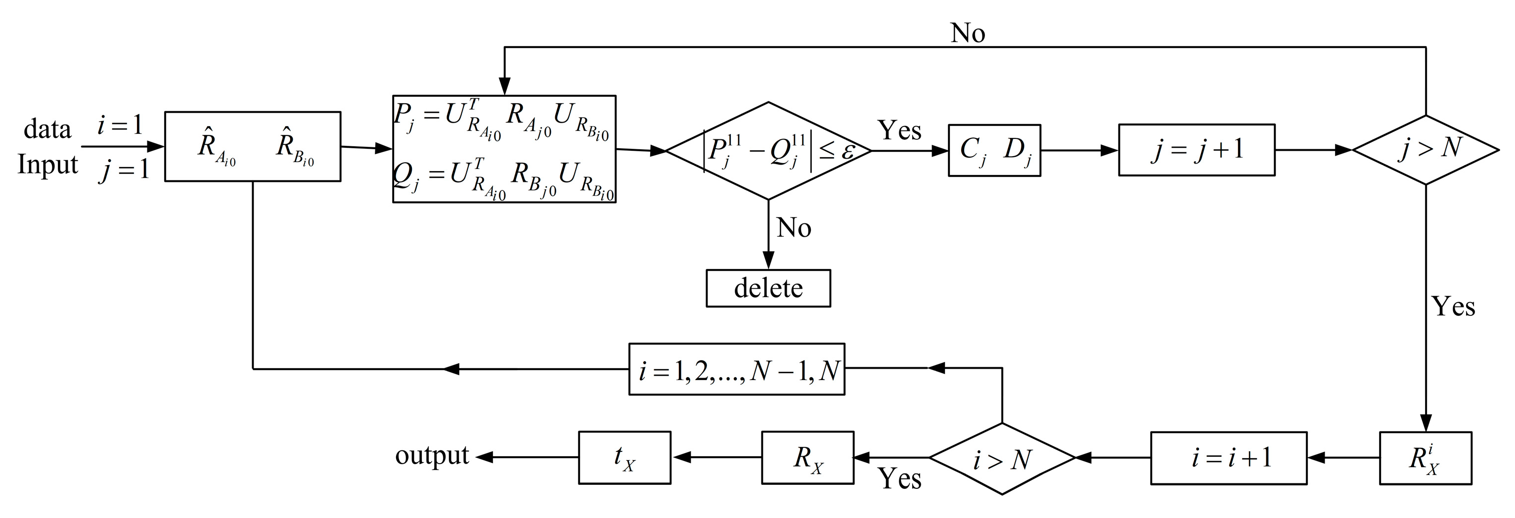
3.3. Outlier Detection

In practice, matrices A_i and B_i contain an observation error, notated as ${\widehat{A}}_i$ and ${\widehat{B}}_i$, respectively. B_i is more sensitive to image noises. A poor environment may lead to a large observation error and, in this case, the global optimization solution has no significance. This is a basic problem that considerably decreases the robustness of hand–eye calibration and has not been well solved.

The form of Y is:

$$Y=\left[\begin{array}{ccc}\pm 1& 0& 0\\ 0& c& d\\ 0& -d& c\end{array}\right]$$

(34)

$R_{A_{i0}}$ and $R_{B_{i0}}$ must satisfy Equation (13).

$$P_i=\left[\begin{array}{ccc}{P}_i^{11}& P_i^{12}& P_i^{13}\\ P_i^{21}& P_i^{22}& P_i^{23}\\ P_i^{31}& P_i^{32}& P_i^{33}\end{array}\right],\hspace{1em}{Q}_i=\left[\begin{array}{ccc}{Q}_i^{11}& Q_i^{12}& Q_i^{13}\\ Q_i^{21}& Q_i^{22}& Q_i^{23}\\ Q_i^{31}& Q_i^{32}& Q_i^{33}\end{array}\right]$$

(35)

For arbitrary c and d, Equation (36) is satisfied:

$$\left|P_i^{11}-Q_i^{11}\right|\le \epsilon$$

(36)

which can be used to discriminate the quality of the observation data: if greater than a specific threshold ε, then the observation data are outliers and should be deleted. The threshold ε is an empirical value. Through setting its value, the observation data can be filtered. The lower the threshold ε, the higher the quality of the observation data. In simulations and experiments, ε was set to 0.01. In summary, the flowchart of the proposed method is described in Figure 2.

3.4. Unique Solution Conditions

Assume the rotation matrices of two movements are A₁, A₂, B₁, and B₂, and X is known. From Theorem 1 (Appendix A), the general solution of A₁X = XB₁ is:

$$X=U_{A_1}Y{U}_{B_1}^T$$

(37)

where, Y is a matric only related to c and d. Substitute Equation (37) into the equation built by two movements:

$$A_{1}X=X{B}_1,A_{2}X=X{B}_2$$

(38)

Substitute them into Equation (13) to obtain:

$$\{\begin{array}{l}{P}_{1}Y=Y{Q}_1\\ P_{2}Y=Y{Q}_2\end{array}$$

(39)

And

$$P_1=Q_1$$

(40)

For Equation (39):

$$rank\left(C_1^T{C}_1\right)=rank\left(\left[\begin{array}{cc}{C}_1^T{C}_1& C_1^T{D}_1\end{array}\right]\right)=0$$

(41)

Equation (41) is an identical equation.

If rotation axes of two movements are not parallel, P₂ and Q₂ are independent:

$$rank\left(C_2^T{C}_2\right)=rank\left(\left[\begin{array}{cc}{C}_2^T{C}_2& C_2^T{D}_2\end{array}\right]\right)=2$$

(42)

From Theorem 2 proved in the Appendix A, if the rotation axes of N movements of the robot gripper are parallel, there will be multiple solutions to the hand–eye calibration. Therefore, the minimal configuration of the unique solution is that the robot gripper and camera move at least twice, and the rotation axes cannot be parallel.

4. Results

4.1. Simulations

We designed simulations to test the performance of different hand–eye calibration methods. The hand–eye calibration equation can be written as:

$$A_{ij}X=X{B}_{ij}$$

(43)

where, A_ij and B_ij are the movement of the robot gripper and camera from time i to time j, respectively. A_i and B_i were simulated as the observation data. X is simulated as the transformation from the camera to the robot gripper. A_i, B_i and X consist of rotation matrices and translation vectors. The rotation matric can be generated using three Euler angles.

The simulations included three parts: analysis of noise sensitivity, relationship between the number of movements and accuracy, and outlier detection ability. All the simulations were performed using MATLAB. In addition to the proposed method, we selected another five popular methods for comparisons [7,11,12,13,23]. For the ith simulation, ${\tilde{R}}_X^i$ and ${\tilde{t}}_X^i$ are the ideal transformation from the camera to the robot gripper and ${\widehat{R}}_X^i$ and ${\widehat{t}}_X^i$ are the measured transformations. The error matric can be calculated as:

$$\begin{array}{l}{R}_{error}^i={\left({\widehat{R}}_X^i\right)}^T{\tilde{R}}_X^i\\ t_{error}^i={\widehat{t}}_X^i-{\tilde{t}}_X^i\end{array}$$

(44)

where, $k_{error}^i$ and ${\theta }_{error}^i$ are the rotation axis and rotation angle of $R_{error}^i$, respectively.

$$\left(k_{error}^i,{\theta }_{error}^i\right)=rodrigues\left(R_{error}^i\right)$$

(45)

The errors of rotation and translation are defined as:

$$\begin{array}{l}{\theta }_{error}=RMS\left({\theta }_{error}^1,{\theta }_{error}^2,\dots ,{\theta }_{error}^{n-1},{\theta }_{error}^n\right)\\ t_{error}=RMS\left(t_{error}^1,t_{error}^2,\dots ,t_{error}^{n-1},t_{error}^n\right)\end{array}$$

(46)

where, n is the number of simulations.

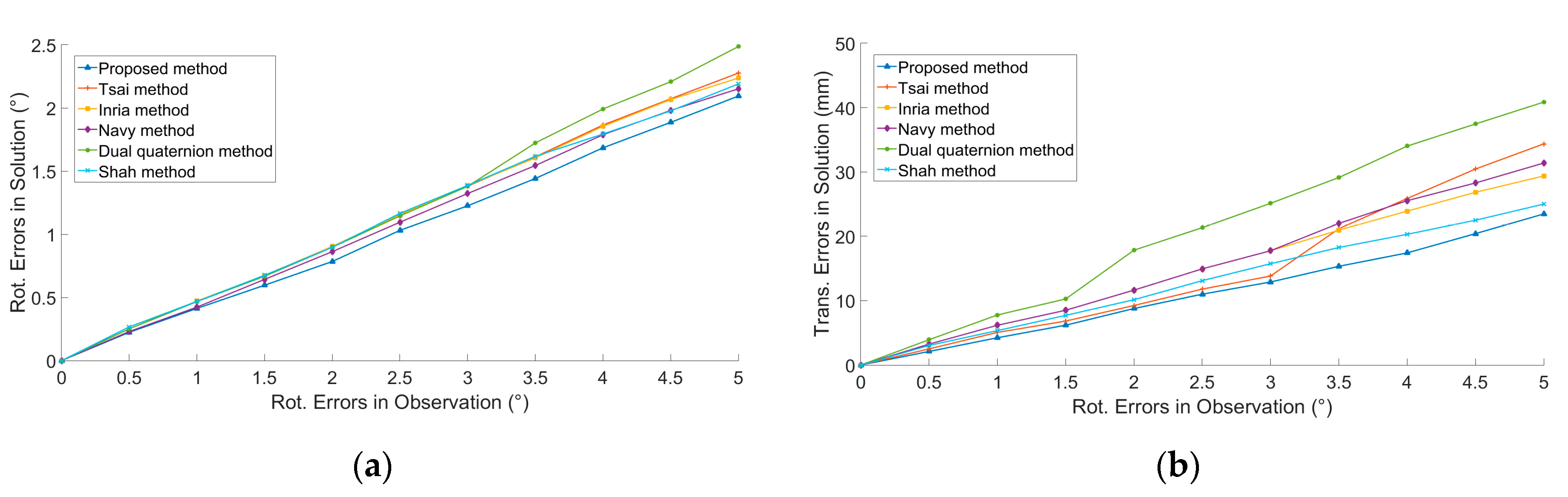
4.1.1. Analysis of Noise Sensitivity

Gaussian rotation noise (μ_R = 0, σ_R = 0°–5°) and translation noise (μ_T = 0, σ_T = 0–5 mm) were added into A_i and B_i (i = 1, 2, …, 9, 10). We ran 100 simulations at each noise level. The results were shown in Figure 3, in which ‘Rot.’ represents ‘Rotation’ and ‘Trans.’ represents ‘Translation’. Except for the dual quaternion method, translation perturbation had no effect on the rotation solution, because only the dual quaternion method solves rotation and translation simultaneously, whereas other methods solve rotation and translation by steps.

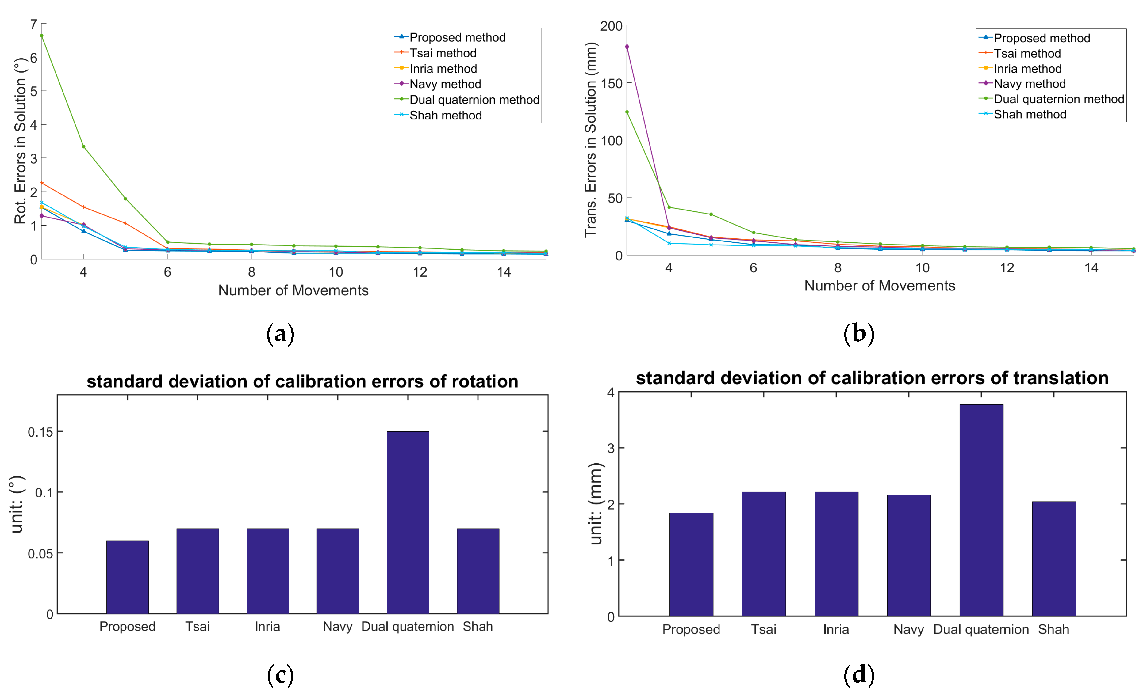
4.1.2. Relationship between Number of Movements and Accuracy

The simulation conditions included σ_R = 0.2°, σ_T = 2 mm, and the number of movements varied from 3 to 15. We ran 100 simulations at each number of movements. Figure 4a,b indicates that the accuracy of hand–eye calibration improves with the increase in the number of movements. When the number of movements increases from three to eight, the accuracy of hand–eye calibration improves considerably. Figure 4c,d demonstrates that the other five methods are more robust, except for the dual quaternion method being unstable.

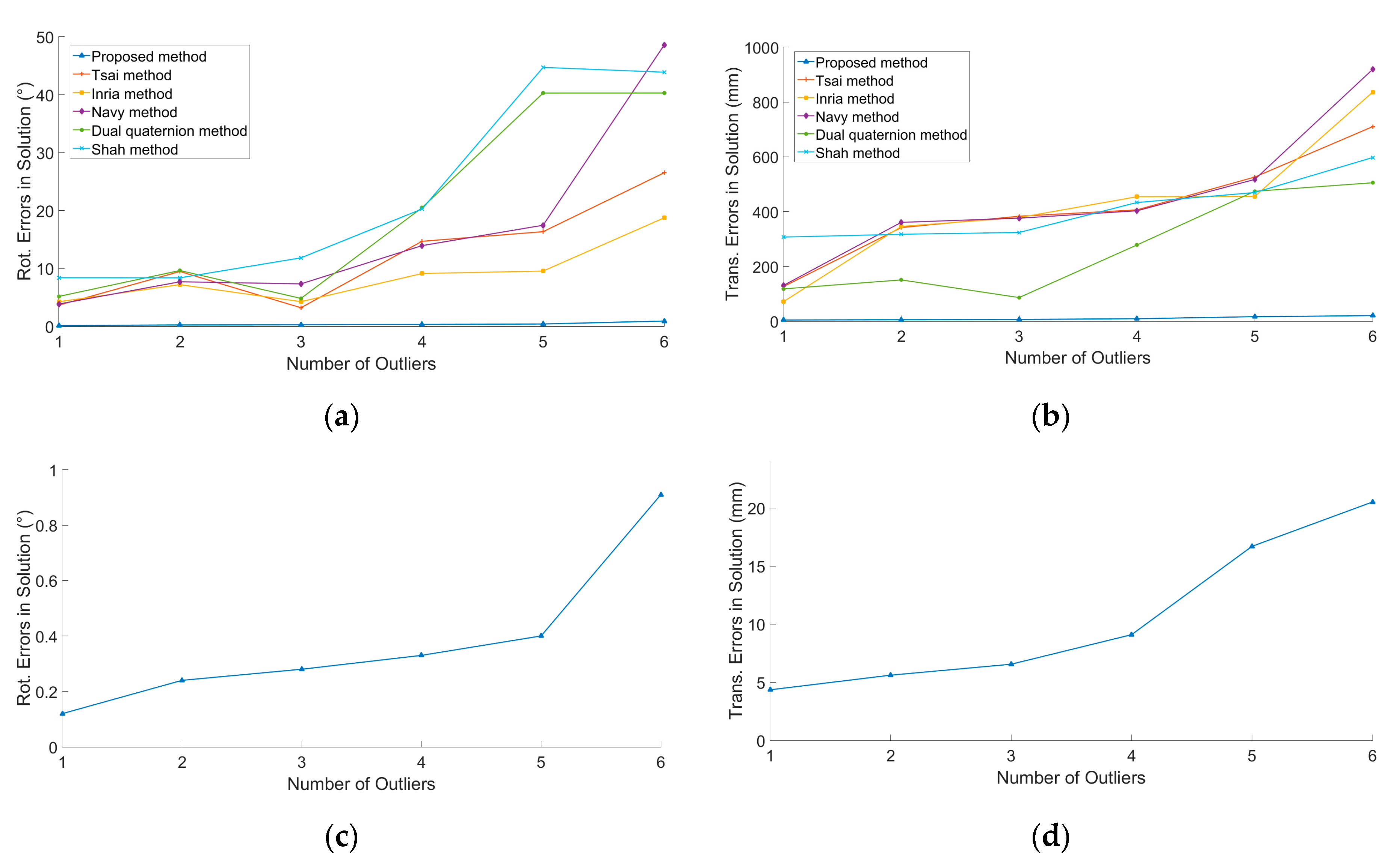
4.1.3. Outlier Detection

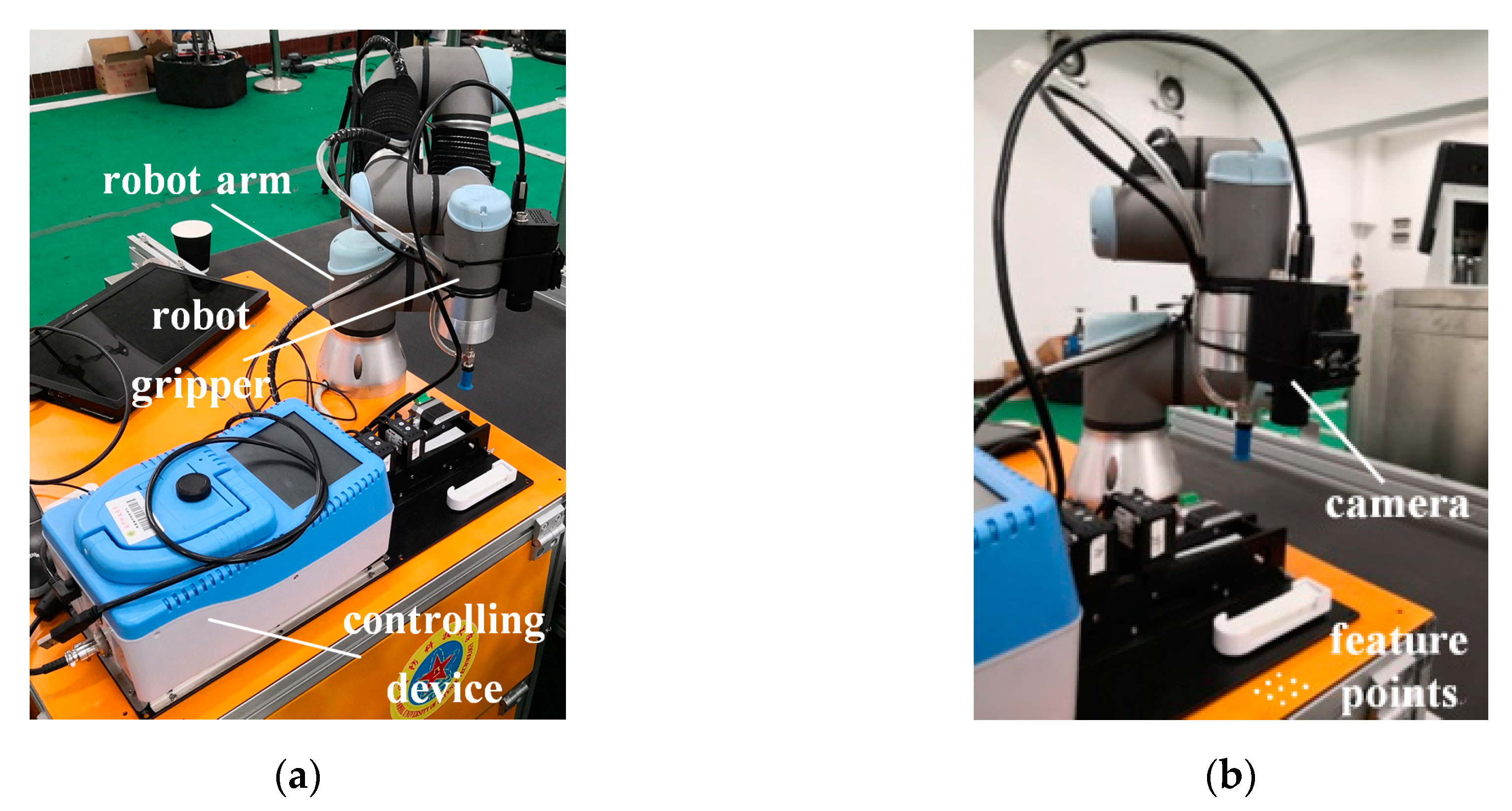
The simulation conditions were σ_R = 0.2°, σ_T = 2 mm, and ε = 0.01. The robot gripper moved 10 times, in which large noise was added into n (n = 1, 2, 3, 4, 5, 6) movements randomly and these observations were regarded as outliers. We ran 100 simulations at each number of outliers. Figure 5a,b shows the relationship between calibration errors of R_X and t_X and the number of outliers, respectively. Figure 5c,d depicts the performance of the proposed method. The results indicate that the proposed method can detect outliers effectively and performs much better than the other five methods.

4.2. Experiments

Determining poses of the robot gripper with high precision is costly, but movements of the robot gripper can be measured precisely. Thus, most researchers adopt the following program to validate hand–eye calibration methods: the camera moves N + n times, where the preview N times are called the calibration link and the last n times are called the verification link. The calibration link is used to solve the transformation between the robot gripper and the camera. The verification link is used to verify method accuracy by comparing its predicted movements with its true movements [3]. The predicted movements of the robot gripper can be solved from the camera’s movements using Equation (47). The true movements of the robot gripper can be obtained from its controlling device. A robot arm was fixed with a camera, as shown in Figure 6a.

For the calibration link:

(1) Fix 9 feature points on the platform as shown in Figure 6b. The three-dimensional (3D) coordinates of feature points can be measured by Leica Total Station. All the feature points’ coordinates remain unchanged during the experiment.

(2) At time 0, capture an image of the feature points on the platform. Calculate the camera’s pose B₀ through Perspective-n-Points (PnP) methods. The robot gripper’s pose A₀ can be determined from its controlling device.

(3) At time i, move the robot gripper and camera.

(4) Capture an image of the feature points on the platform. Calculate the camera’s pose B_i through PnP methods. The robot gripper’s pose A_i can be determined from its controlling device.

(5) Repeat step (3)–(4) N times and (A_i0, B_i0) (i = 1, …, N–1, N) can be obtained.

(6) The transformation X from the camera to the robot gripper can be calibrated using all six hand–eye calibration methods.

For the verification link:

(7) Repeat step (3)–(4) n times and (A_i0, B_i0) (i = N+1, …, N+n–1, N+n) can be obtained.

(8) The predicted movement ${\widehat{A}}_{i0}$ of the robot gripper can be calculated through Equation (47). The true movement of the robot gripper A_i0 can be obtained from its controlling device.

$${\widehat{A}}_{i0}=X{B}_{i0}{X}^{-1}$$

(47)

(9) Comparing ${\widehat{A}}_{i0}$ with A_i0, the error matric can be calculated using Equation (48):

$$\begin{array}{l}{R}_{error}^i={\left({\widehat{R}}_{A_{i0}}\right)}^T{R}_{A_{i0}}\\ t_{error}^i={\widehat{t}}_{A_{i0}}-t_{A_{i0}}\end{array}$$

(48)

$k_{error}^i$ and ${\theta }_{error}^i$ are the corresponding rotation axis and rotation angle of $R_{error}^i$, respectively:

$$\left(k_{error}^i,{\theta }_{error}^i\right)=rodrigues\left(R_{error}^i\right)$$

(49)

The rotation and translation errors are defined as:

$$\begin{array}{l}{\theta }_{error}=RMS\left({\theta }_{error}^1,{\theta }_{error}^2,\dots ,{\theta }_{error}^{n-1},{\theta }_{error}^n\right)\\ t_{error}=RMS\left(t_{error}^1,t_{error}^2,\dots ,t_{error}^{n-1},t_{error}^n\right)\end{array}$$

(50)

The rotation error is in arcmin and the translation error is in mm.

In the experiment, N = 2–9 and n = 200. The results are shown in

Table 1. Prediction error: t_error in mm and θ_error in arcmin.

N	Proposed		Tsai		Inria		Navy		Dual Quaternion		Shah
	θerror	terror	θerror	terror	θerror	terror	θerror	terror	θerror	terror	θerror	terror
2	10.14	5.49	10.14	7.06	10.14	6.23	10.17	5.25	10.21	8.70	10.14	5.63
3	10.10	4.63	10.10	6.21	10.14	6.20	10.14	5.10	10.14	7.08	10.10	4.71
4	10.07	4.06	10.10	5.77	10.10	4.74	10.10	4.97	10.14	6.18	10.10	4.16
5	9.83	3.94	10.07	4.15	10.07	3.79	10.07	4.62	10.10	4.17	9.86	4.04
6	0.96	2.46	0.96	3.67	1.30	3.61	2.16	3.54	3.81	3.98	1.34	2.60
7	0.44	1.57	0.51	3.51	0.51	3.60	0.51	1.87	1.78	3.64	0.72	1.75
8	0.37	1.15	0.37	2.76	0.41	2.51	0.44	1.77	0.44	2.27	0.37	1.20
9	0.06	1.01	0.27	2.47	0.34	2.27	0.41	1.19	0.41	1.82	0.20	1.05

. The experiment results indicate that the prediction error decreased with the increase in the number of movements and when the robot gripper moved 9 times, the proposed method’s prediction accuracy of rotation exceeded 6 arcsec, which is much higher than the calibration accuracy in the simulations. The reason is explained in the following.

Expand Equation (47) using a partition matric:

$${\widehat{R}}_{A_{i0}}=R_X{R}_{B_{i0}}{R}_X^{-1}$$

(51)

The prediction error consists of hand–eye calibration error and camera pose estimation error. Hand–eye calibration error is notated as ∆R_X. Then, the prediction error of Equation (51) can be written as:

$$e={\Vert R_X\mathsf{\Delta }{R}_X{R}_{B_{i0}}\mathsf{\Delta }{R}_X^{-1}{R}_X^{-1}-R_X{R}_{B_{i0}}{R}_X^{-1}\Vert }_F\le \lambda {\Vert \mathsf{\Delta }{R}_X{R}_{B_{i0}}\mathsf{\Delta }{R}_X^{-1}-R_{B_{i0}}\Vert }_F$$

(52)

Equation (52) can weaken the effect of the hand–eye calibration error. This conclusion also applies to the prediction error of translation. Thus, the prediction error in the experiment was much lower than the hand–eye calibration error in the simulations.

5. Conclusions

A hand–eye calibration method with high accuracy and robustness was proposed in this paper. Using this method, the basic problem of observation data preprocessing is solved by outlier detection, which significantly improves robustness. However, two aspects remain to be studied. To improve the method’s efficiency, we used the least squares optimization method with constraints. If no strict need exists for efficiency, an iterative method could be considered. We decreased the rotation matric’s dimension from three to two via Schur matric decomposition and unknown parameters satisfied the constraint c² + d² = 1. If the following triangle transformation is adopted, the degrees of freedom (DOFs) can be decreased from two to one. The Gröbner basis method can be used to solve polynomial equations [24]:

$$c=\frac{2\tan \frac{\theta }{2}}{1+{\tan }^2\frac{\theta }{2}},d=\frac{1-{\tan }^2\frac{\theta }{2}}{1+{\tan }^2\frac{\theta }{2}}$$

(53)

References

1. Knight, J.; Reid, I. Automated alignment of robotic pan-tilt camera units using vision. Int. J. Comput. Vis. 2006, 68, 219–237. [Google Scholar] [CrossRef]
2. Eschelbach, M.; Aghaeifar, A.; Bause, J.; Handwerker, J.; Anders, J.; Engel, E.M.; Thielscher, A.; Scheffler, K. Comparison of prospective head motion correction with NMR field probes and an optical tracking system. Magn. Reson. Med. 2018, 81, 719–729. [Google Scholar] [CrossRef] [PubMed] [Green Version]
3. Song, Y.; Zhang, J.; Lian, B.; Sun, T. Kinematic calibration of a 5-DOF parallel kinematic machine. Precis. Eng. 2016, 45, 242–261. [Google Scholar] [CrossRef]
4. Pan, H.; Wang, N.L.; Qin, Y.S. A closed-form solution to eye-to-hand calibration towards visual grasping. Ind. Robot 2014, 41, 567–574. [Google Scholar] [CrossRef]
5. Ali, I.; Suominen, O.; Gotchev, A.; Morales, E.R. Methods for simultaneous robot-world-hand-eye calibration: A comparative study. Sensors 2019, 19, 2837. [Google Scholar] [CrossRef]
6. Shiu, Y.C.; Ahmad, S. Calibration of wrist-mounted robotic sensors by solving homogeneous transform equations of the form AX = XB. IEEE Trans. Robot. Autom. 1989, 5, 16–29. [Google Scholar] [CrossRef]
7. Tsai, R.Y.; Lenz, R.K. A new technique for fully autonomous and efficient 3D robotics hand-eye calibration. IEEE Trans. Robot. Autom. 1989, 5, 345–358. [Google Scholar] [CrossRef]
8. Wang, Z.; Liu, Z.; Ma, Q.; Cheng, A.; Liu, Y.H.; Kim, S.; Deguet, A.; Reiter, A.; Kazanzides, P.; Taylor, R.H. Vision-based calibration of dual RCM-based robot arms in human-robot collaborative minimally invasive surgery. IEEE Robot. Autom. Lett. 2017, 3, 672–679. [Google Scholar] [CrossRef]
9. Zhang, Z.Q.; Zhang, L.; Yang, G.Z. A computationally efficient method for hand-eye calibration. Int. J. Comput. Assist. Radiol. Surg. 2017, 12. [Google Scholar] [CrossRef]
10. Li, H.; Ma, Q.; Wang, T.; Chirikjian, G.S. Simultaneous hand-eye and robot-world calibration by solving the AX = XB problem without correspondence. IEEE Robot. Autom. Lett. 2015, 8, 145–152. [Google Scholar] [CrossRef]
11. Daniilidis, K. Hand-eye calibration using dual quaternions. Int. J. Robot. Res. 1999, 18, 286–298. [Google Scholar] [CrossRef]
12. Park, F.C.; Martin, B.J. Robot sensor calibration: Solving AX = XB on the Euclidean group. IEEE Trans. Robot. Autom. Lett. 1994, 10, 717–721. [Google Scholar] [CrossRef]
13. Shah, M. Solving the robot-world/hand-eye calibration problem using the Kronecker product. J. Mech. Robot. 2013, 5, 031007. [Google Scholar] [CrossRef]
14. Pachtrachai, K.; Vasconcelos, F.; Chadebecq, F.; Allan, M.; Hailes, S.; Pawar, V.; Stoyanov, D. Adjoint transformation method for hand-eye calibration with applications in robotics assisted surgery. Ann. Biomed. Eng. 2018, 46, 1606–1620. [Google Scholar] [CrossRef]
15. Fassi, I.; Legnani, G. Hand to sensor calibration: A geometrical interpretation of the matric equation AX = XB. J. Robot. Syst. 2005, 22, 497–506. [Google Scholar] [CrossRef]
16. Li, W.; Dong, M.L.; Lu, N.G. Simultaneous robot-world and hand-eye calibration without a calibration object. Sensors 2018, 18, 3949. [Google Scholar] [CrossRef]
17. Cao, C.T.; Do, V.P.; Lee, B.Y. A novel indirect calibration approach for robot positioning error compensation based on neural network and hand-eye vision. Appl. Sci. 2019, 9, 1940. [Google Scholar] [CrossRef]
18. Ruland, T.; Pajdla, T.; Kruger, L. Robust hand-eye self-calibration. In Proceedings of the IEEE Conference on Intelligent Transportation Systems, Washington, DC, USA, 5–7 October 2011; pp. 87–94. [Google Scholar] [CrossRef]
19. Schmidt, J.; Niemann, H. Data-selection for hand–eye calibration: A vector quantization approach. Int. J. Robot. Res. 2008, 27, 1027–1053. [Google Scholar] [CrossRef]
20. Shu, T.; Zhang, B.; Tang, Y.Y. Multi-view classification via a fast and effective multi-view nearest-subspace classifier. IEEE Access 2019, 7, 49669–49679. [Google Scholar] [CrossRef]
21. Adachi, S.; Iwata, S.; Nakatsukasa, Y.; Takeda, A. Solving the trust-region subproblem by a generalized eigenvalue problem. SIAM J. Optim. 2017, 27, 269–291. [Google Scholar] [CrossRef]
22. Park, Y.; Gerstoft, P.; Seonng, W. Grid-free compressive mode extraction. J. Acoust. Soc. Am. 2019, 145, 1427–1442. [Google Scholar] [CrossRef] [PubMed]
23. Horaud, R.; Dornaika, F. Hand-eye calibration. Int. J. Robot. Res. 1995, 14, 195–210. [Google Scholar] [CrossRef]
24. Xu, C.; Zhang, L.H.; Cheng, L. Pose estimation from line correspondences: A complete analysis and a series of solutions. IEEE Trans. Pattern Anal. Mach. Intell. 2016, 39, 1209–1222. [Google Scholar] [CrossRef] [PubMed]
Figure 1. Description of the hand–eye calibration problem.
Sensors 19 04490 g001
Figure 2. Flowchart of the proposed method.
Sensors 19 04490 g002
Figure 3. The relationship between calibration accuracy and observation errors: (a) Rotation errors in observations and calibration errors of RX. (b) Rotation errors in observations and calibration errors of tX. (c) Translation errors in observations and calibration errors of RX. (d) Translation errors in observation and calibration errors of tX. Each point on the figure is the Root Mean Square (RMS) of 100 simulations.
Sensors 19 04490 g003aSensors 19 04490 g003b
Figure 4. The relationship between calibration accuracy and the number of movements: (a) The number of movements and the calibration errors of RX. (b) The number of movements and the calibration errors of tX. (c) The standard deviations of the calibration errors of RX. (d) The standard deviations of the calibration errors of tX. Each point on the figure is the RMS of 100 simulations.
Sensors 19 04490 g004
Figure 5. The relationship between calibration accuracy and the number of outliers: (a) Calibration errors of RX and the number of outliers. (b) Calibration errors of tX and the number of outliers. (c) Partial enlargers of (a). (d) Partial enlargers of (b). Each point on the figure is the RMS of 100 simulations.
Sensors 19 04490 g005
Figure 6. (a) Robot arm, gripper and its controlling device. (b) Camera and feature points.
Sensors 19 04490 g006