Evaluation of Aboveground Nitrogen Content of Winter Wheat Using Digital Imagery of Unmanned Aerial Vehicles

 ,
, 
 ,
,
Abstract
1. Introduction
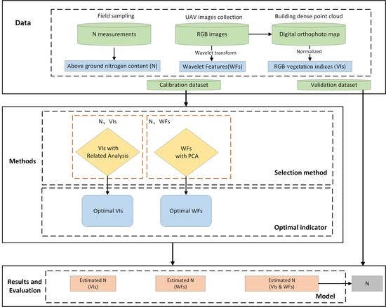
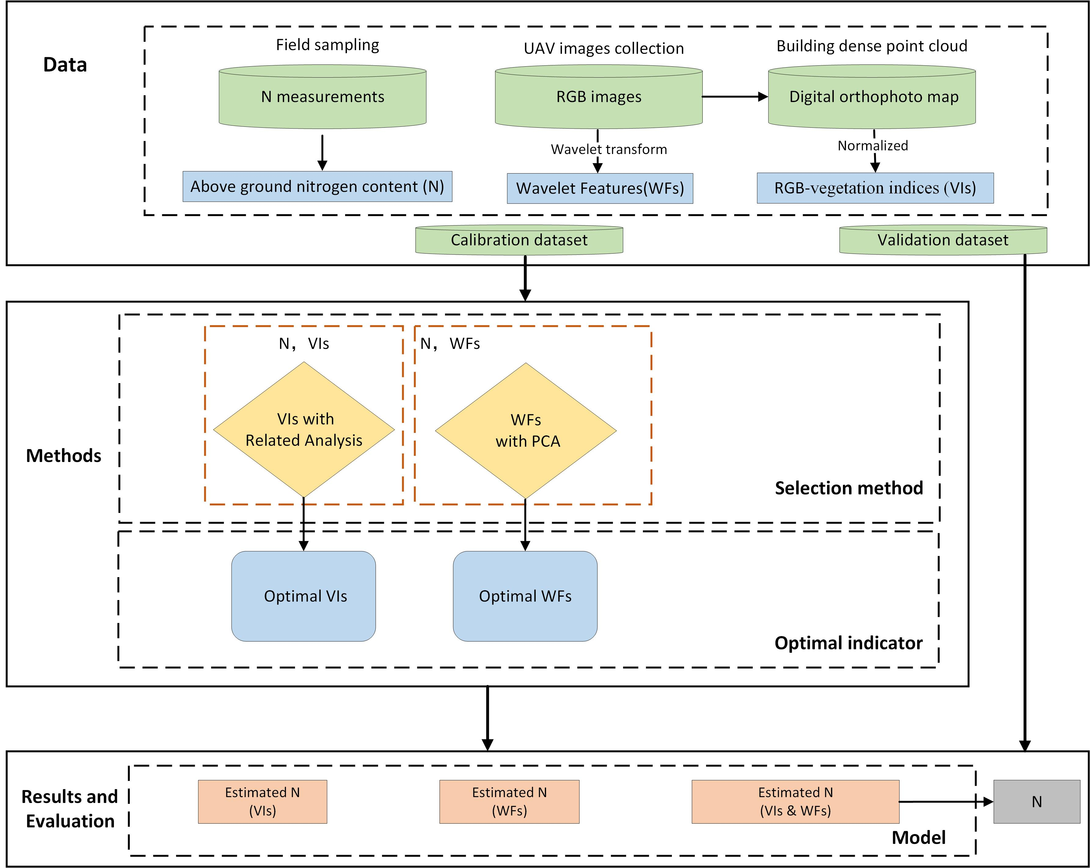
2. Data and Methods
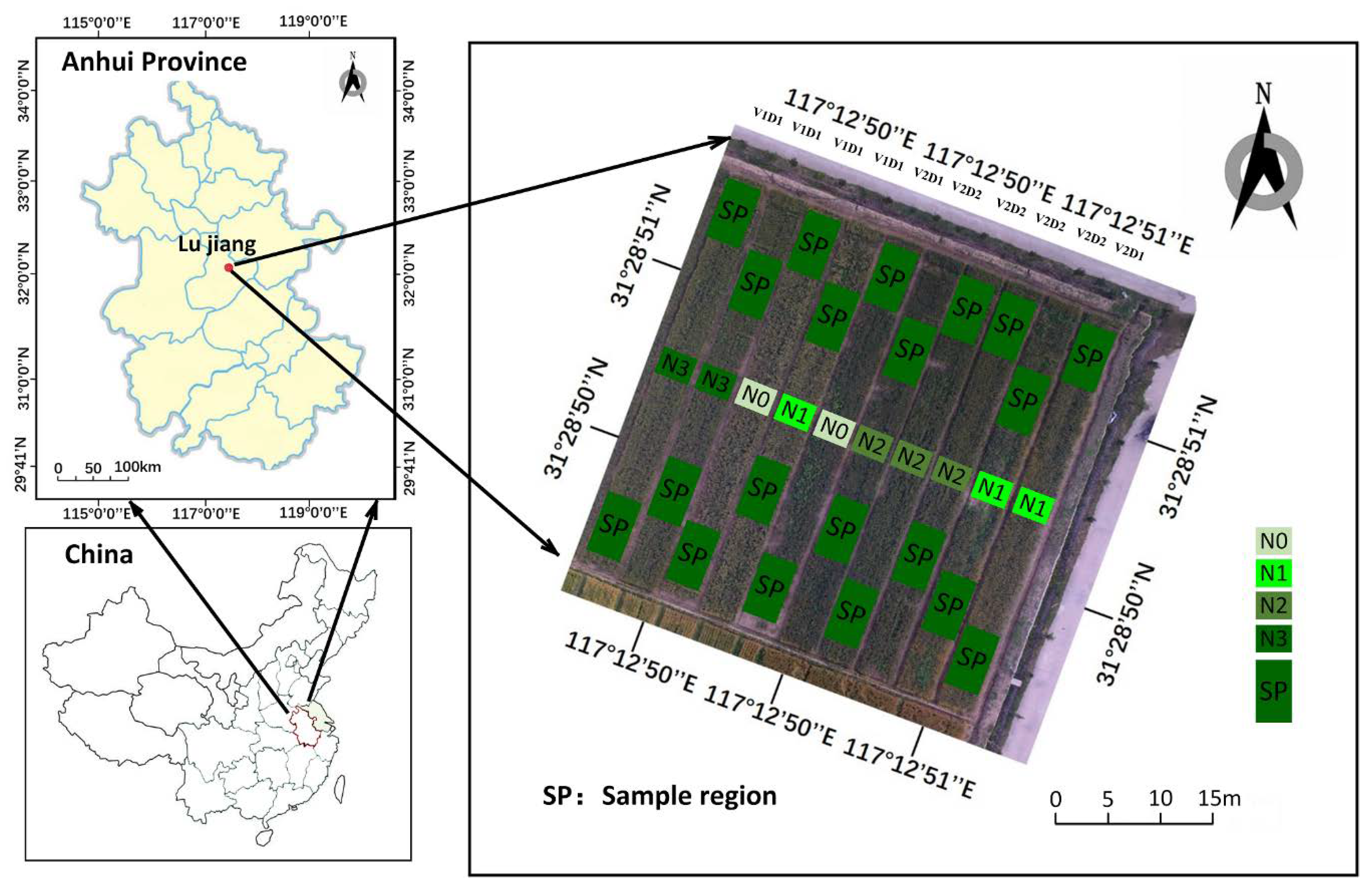
2.1. Experimental Design
2.2. Data Collection
2.3. Feature Extraction
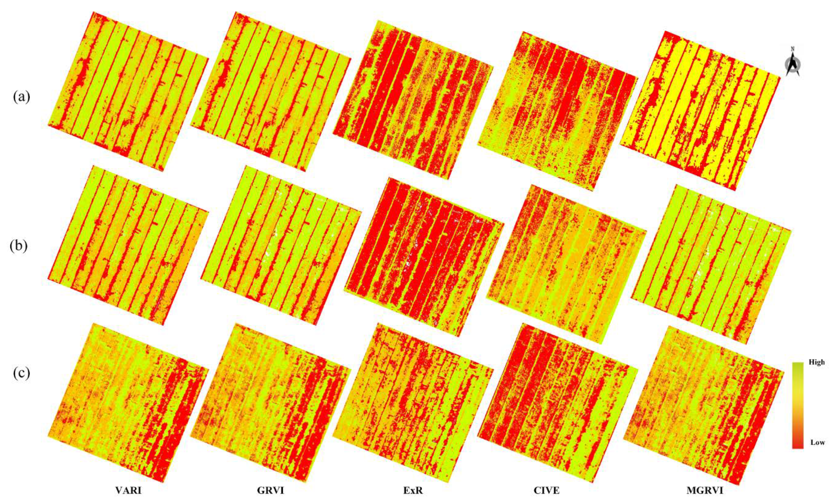
2.3.1. Vegetation Indices
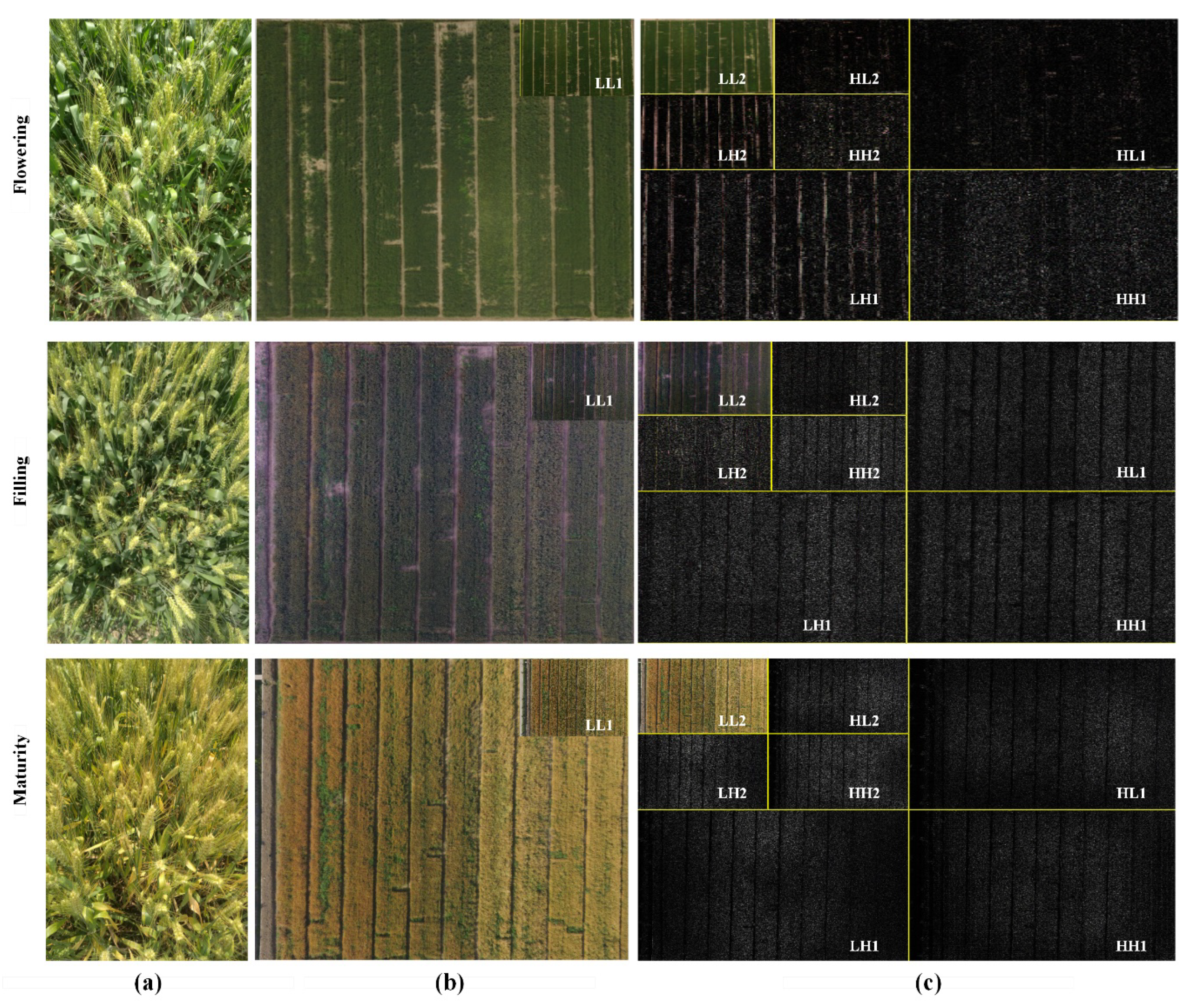
2.3.2. Wavelet Features
2.4. Methods
2.4.1. Related Technologies
2.4.2. Model Validation
3. Results and Analysis
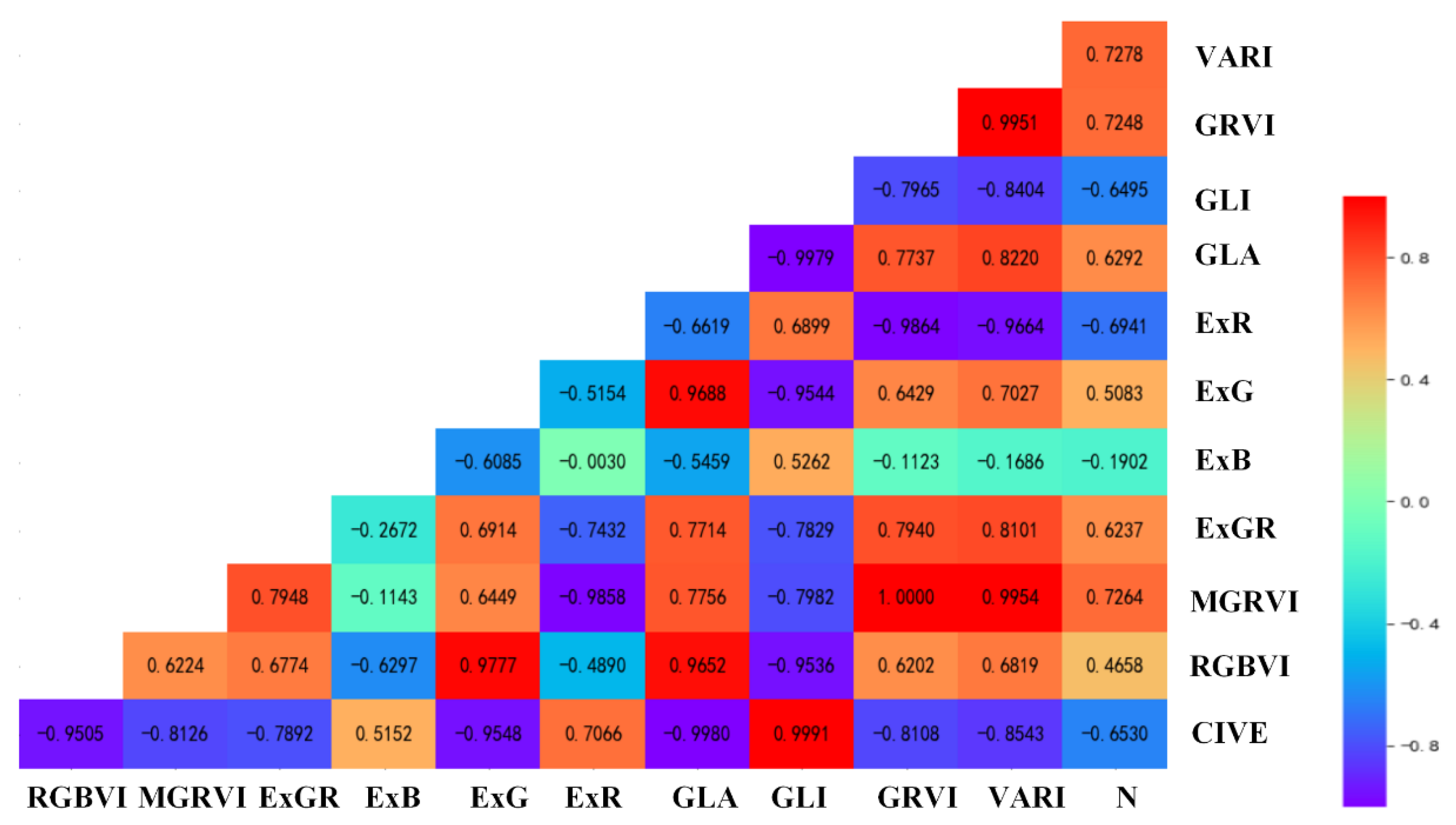
3.1. Correlation Analysis between Vegetation Indices and Aboveground Nitrogen Content of Wheat
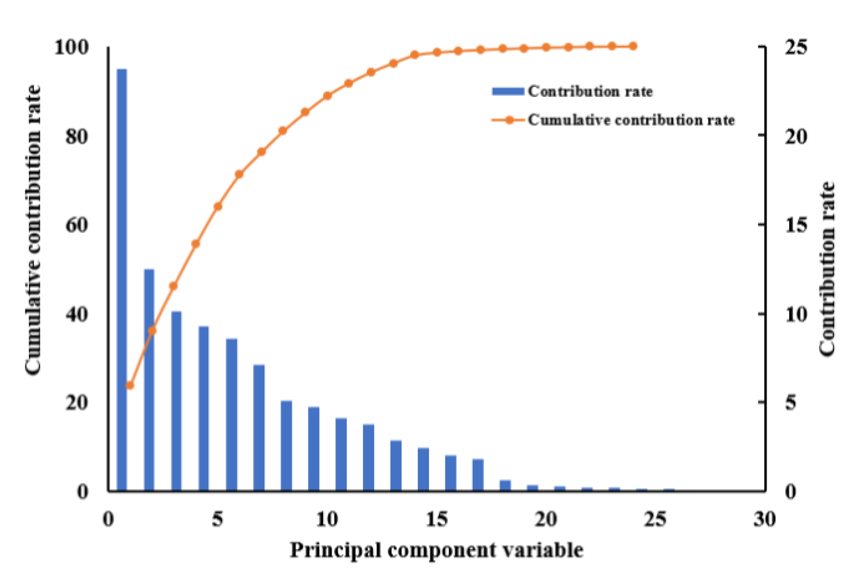
3.2. Extraction and Analysis of Wavelet Features
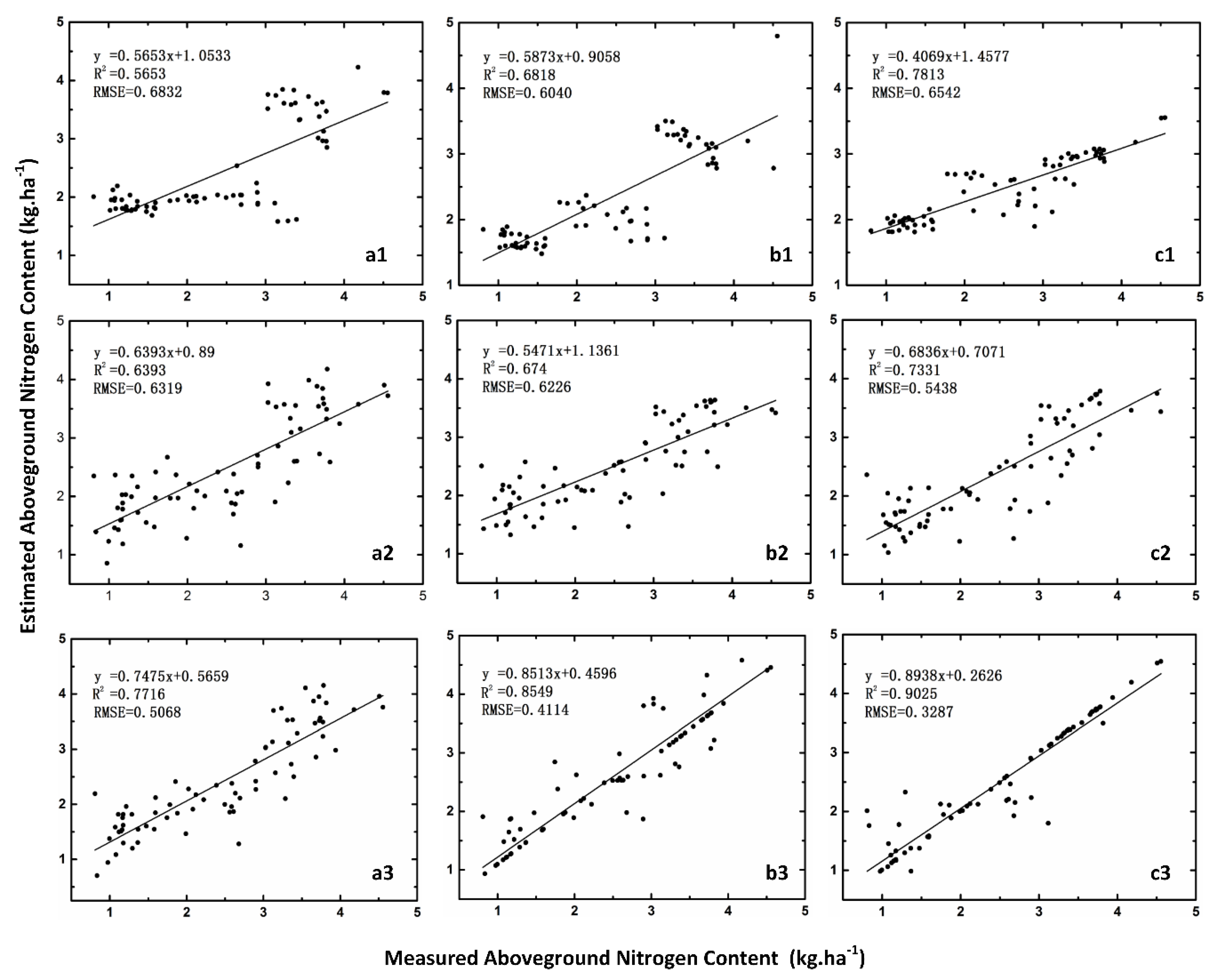
3.3. Performance of Models Based on Different Methods
3.4. Performance Based on Different Feature Variables
4. Discussion
4.1. Vegetation Indices and Wavelet Features
4.2. Spatial Resolution and Wavelet Transform
4.3. Comparison of Feature Selection Methods
4.4. Comparison of PLS, SVR, and PSO-SVR for Estimating Aboveground Nitrogen Content
5. Conclusions
Supplementary Materials
Supplementary File 1Author Contributions
Funding
Acknowledgments
Conflicts of Interest
References
- Zhu, Y.; Tian, Y.; Yao, X.; Liu, X.; Cao, W. Analysis of Common Canopy Reflectance Spectra for Indicating Leaf Nitrogen Concentrations in Wheat and Rice. Plant Prod. Sci. 2007, 10, 400–411. [Google Scholar] [CrossRef]
- Zhu, Y.; Yao, X.; Tian, Y.; Liu, X.; Cao, W. Evaluation of Six Algorithms to Monitor Wheat Leaf, Nitrogen Concentration. Remote Sens. 2015, 7, 14939–14966. [Google Scholar]
- Zhu, Y.; Yao, X.; Tian, Y.; Liu, X.; Cao, W. Analysis of common canopy vegetation indices for indicating leaf nitrogen accumulations in wheat and rice. Int. J. Appl. Earth Obs. Geoinf. 2008, 10, 1–10. [Google Scholar] [CrossRef]
- Guo, C.; Zhang, L.; Zhou, X.; Zhu, Y.; Cao, W.; Qiu, X.; Tian, Y. Integrating remote sensing information with crop model to monitor wheat growth and yield based on simulation zone partitioning. Precis. Agric. 2017, 19, 55–78. [Google Scholar] [CrossRef]
- Feng, W.; Zhu, Y.; Tian, Y.; Cao, W.; Yao, X.; Liu, Y. Monitoring leaf nitrogen accumulation in wheat with hyper-spectral remote sensing. Acta Ecol. Sin. 2008, 28, 23–32. [Google Scholar]
- Latif, M.A.; Cheema, M.J.M.; Saleem, M.F.; Maqsood, M. Mapping wheat response to variations in N, P, Zn, and irrigation using an unmanned aerial vehicle. Int. J. Remote Sens. 2018, 39, 7172–7188. [Google Scholar] [CrossRef]
- Zecha, C.W.; Peteinatos, G.G.; Link, J.; Claupein, W. Utilisation of Ground and Airborne Optical Sensors for Nitrogen Level Identification and Yield Prediction in Wheat. Agriculture 2018, 8, 79. [Google Scholar] [CrossRef]
- Vincini, M.; Amaducci, S.; Frazzi, E. Empirical Estimation of Leaf Chlorophyll Density in Winter Wheat Canopies Using Sentinel-2 Spectral Resolution. IEEE Trans. Geosci. Remote Sens. 2014, 52, 3220–3235. [Google Scholar] [CrossRef]
- Wang, L.; Tian, Y.; Yao, X.; Zhu, Y.; Cao, W. Predicting grain yield and protein content in wheat by fusing multi-sensor and multi-temporal remote-sensing images. Field Crops Res. 2014, 164, 178–188. [Google Scholar] [CrossRef]
- Kanning, M.; Kühling, I.; Trautz, D.; Jarmer, T. High-resolution UAV-based hyperspectral imagery for LAI and chlorophyll estimations from wheat for yield prediction. Remote Sens. 2018, 10, 2000. [Google Scholar] [CrossRef]
- Zheng, H.; Li, W.; Jiang, J.; Liu, Y.; Cheng, T.; Tian, Y. A comparative assessment of different modeling algorithms for estimating leaf nitrogen content in winter wheat using multispectral images from an unmanned aerial vehicle. Remote Sens. 2018, 10, 2026. [Google Scholar] [CrossRef]
- Duan, T.; Chapman, S.C.; Guo, Y.; Zheng, B. Dynamic monitoring of NDVI in wheat agronomy and breeding trials using an unmanned aerial vehicle. Field Crops Res. 2017, 210, 71–80. [Google Scholar] [CrossRef]
- Liu, H.; Zhu, H.; Wang, P. Quantitative modelling for leaf nitrogen content of winter wheat using UAV-based hyperspectral data. Int. J. Remote Sens. 2016, 38, 1–18. [Google Scholar] [CrossRef]
- Tilly, N.; Aasen, H.; Bareth, G. Fusion of plant height and vegetation indices for the estimation of barley biomass. Remote Sens. 2015, 7, 11449–11480. [Google Scholar] [CrossRef]
- Zhu, H.; Liu, H.; Xu, Y.; Yang, G. UAV-based hyperspectral analysis and spectral indices constructing for quantitatively monitoring leaf nitrogen content of winter wheat. Appl. Opt. 2018, 57, 7722–7732. [Google Scholar] [CrossRef]
- Parraga, A.; Doering, D.; Atkinson, J.G.; Bertani, T.; de Oliveira, A.F.C.; de Souza, M.R.Q.; Susin, A.A. Wheat Plots Segmentation for Experimental Agricultural Field from Visible and Multispectral UAV Imaging. In Proceedings of the SAI Intelligent Systems Conference, London, UK, 6–7 September 2018; pp. 388–399. [Google Scholar]
- Agüera-Vega, F.; Carvajal-Ramírez, F.; Saiz, M.P.; Rosúa, F.O. Multi-temporal imaging using an unmanned aerial vehicle for monitoring a sunflower crop. Biosyst. Eng. 2015, 132, 19–27. [Google Scholar] [CrossRef]
- Yuan, W.; Li, J.; Bhatta, M.; Shi, Y.; Baenziger, P.; Ge, Y. Wheat height estimation using lidar in comparison to ultrasonic sensor and UAS. Sensors 2018, 18, 3731. [Google Scholar] [CrossRef]
- Liu, Y.; Cheng, T.; Zhu, Y.; Tian, Y.; Cao, W.; Yao, X.; Wang, N. Comparative analysis of vegetation indices, non-parametric and physical retrieval methods for monitoring nitrogen in wheat using UAV-based multispectral imagery. In 2016 IEEE International Geoscience and Remote Sensing Symposium (IGARSS); IEEE: Beijing, China, 2016; pp. 7362–7365. [Google Scholar]
- Eitel, J.U.; Magney, T.S.; Vierling, L.A.; Brown, T.T.; Huggins, D.R. LiDAR based biomass and crop nitrogen estimates for rapid, non-destructive assessment of wheat nitrogen status. Field Crops Res. 2014, 159, 21–32. [Google Scholar] [CrossRef]
- Rasmussen, J.; Nielsen, J.; Garcia-Ruiz, F.; Christensen, S.; Streibig, J.C. Potential uses of small unmanned aircraft systems (UAS) in weed research. Weed Res. 2013, 53, 242–248. [Google Scholar] [CrossRef]
- Lelong, C.C.D.; Burger, P.; Jubelin, G.; Roux, B.; Labbé, S.; Baret, F. Assessment of unmanned aerial vehicles imagery for quantitative monitoring of wheat crop in small plots. Sensors 2008, 8, 3557–3585. [Google Scholar] [CrossRef]
- Mathews, A.; Jensen, J. Visualizing and quantifying vineyard canopy LAI using an Unmanned Aerial Vehicle (UAV) collected high density structure from motion point cloud. Remote Sens. 2013, 5, 2164–2183. [Google Scholar] [CrossRef]
- Tanaka, S.; Kawamura, K.; Maki, M.; Muramoto, Y.; Yoshida, K.; Akiyama, T. Spectral Index for Quantifying Leaf Area Index of Winter Wheat by Field Hyperspectral Measurements: A Case Study in Gifu Prefecture, Central Japan. Remote Sens. 2015, 7, 5329–5346. [Google Scholar] [CrossRef]
- Verger, A.; Vigneau, N.; Chéron, C.; Gilliot, J.M.; Comar, A.; Baret, F. Green area index from an unmanned aerial system over wheat and rapeseed crops. Remote Sens. Environ. 2014, 152, 654–664. [Google Scholar] [CrossRef]
- Bendig, J.; Bolten, A.; Bareth, G. UAV-based imaging for multi-temporal, very high resolution crop surface models to monitor crop growth variability. Photogramm. Fernerkund. Geoinf. 2013, 6, 551–562. [Google Scholar] [CrossRef]
- Bendig, J.; Bolten, A.; Bennertz, S.; Broscheit, J.; Eichfuss, S.; Bareth, G. Estimating biomass of barley using Crop Surface Models (CSMs) derived from UAV-based RGB imaging. Remote Sens. 2014, 6, 10395–10412. [Google Scholar] [CrossRef]
- Pölönen, I.; Saari, H.; Kaivosoja, J.; Honkavaara, E.; Pesonen, L. Hyperspectral imaging based biomass and nitrogen content estimations from light-weight UAV. In Proceedings of the SPIE 8887, Remote Sensing for Agriculture, Ecosystems, and Hydrology XV, 88870J, Dresden, Germany, 23–26 September 2013; pp. 521–525. [Google Scholar]
- Honkavaara, E.; Saari, H.; Kaivosoja, J.; Pölönen, I.; Hakala, T.; Litkey, P.; Mäkynen, J.; Pesonen, L. Processing and assessment of spectrometric, stereoscopic imagery collected using a lightweight UAV spectral camera for precision agriculture. Remote Sens. 2013, 5, 5006–5039. [Google Scholar] [CrossRef]
- Possoch, M.; Bieker, S.; Hoffmeister, D.; Bolten, A.; Schellberg, J.; Bareth, G. Multi-temporal crop surface models combined with the RGB vegetation index from UAV-based images for forage monitoring in grassland. Int. Arch. Photogramm. Remote Sens. Spat. Inf. Sci. 2016, 41, 991–998. [Google Scholar] [CrossRef]
- Schirrmann, M.; Giebel, A.; Gleiniger, F.; Pflanz, M.; Lentschke, J.; Dammer, K.H. Monitoring agronomic parameters of winter wheat crops with low-cost UAV imagery. Remote Sens. 2016, 8, 706. [Google Scholar] [CrossRef]
- Øvergaard, S.I.; Isaksson, T.; Kvaal, K.; Korsaeth, A. Comparisons of two hand-held, multispectral field radiometers and a hyperspectral airborne imager in terms of predicting spring wheat grain yield and quality by means of powered partial least squares regression. J. Near Infrared Spectrosc. 2010, 18, 247–261. [Google Scholar] [CrossRef]
- Rasmussen, J.; Ntakos, G.; Nielsen, J.; Svensgaard, J.; Poulsen, R.N.; Christensen, S. Are vegetation indices derived from consumer-grade cameras mounted on UAVs sufficiently reliable for assessing experimental plots? Eur. J. Agron. 2016, 74, 75–92. [Google Scholar] [CrossRef]
- Niu, Q.; Feng, H.; Li, C.; Yang, G.; Fu, Y.; Li, Z. Estimation of Leaf Nitrogen Concentration of Winter Wheat Using UAV-Based RGB Imagery. In International Conference on Computer and Computing Technologies in Agriculture; Springer: Cham, Switzerland, 2017; pp. 139–153. [Google Scholar]
- Hunt, E.R.; Hively, W.D.; Fujikawa, S.J.; Linden, D.S.; Daughtry, C.S.T.; McCarty, G.W. Acquisition of NIR-Green-Blue digital photographs from unmanned aircraft for crop monitoring. Remote Sens. 2010, 2, 290–305. [Google Scholar] [CrossRef]
- Corti, M.; Cavalli, D.; Cabassi, G.; Vigoni, A.; Degano, L.; Gallina, P.M. Application of a low-cost camera on a UAV to estimate maize nitrogen-related variables. Precision Agric. 2019, 20, 675–696. [Google Scholar] [CrossRef]
- Geipel, J.; Link, J.; Wirwahn, J.; Claupein, W. A programmable aerial multispectral camera system for in-season crop biomass and nitrogen content estimation. Agriculture 2016, 6, 4. [Google Scholar] [CrossRef]
- Bellens, R.; Gautama, S.; Martinez-Fonte, L.; Philips, W.; Chan, J.C.W.; Canters, F. Improved Classification of VHR Images of Urban Areas Using Directional Morphological Profiles. IEEE Trans. Geosci. Remote Sens. 2008, 46, 2803–2813. [Google Scholar] [CrossRef]
- Yue, J.; Yang, G.; Tian, Q.; Feng, H.; Xu, K.; Zhou, C. Estimate of winter-wheat above-ground biomass based on UAV ultrahigh-ground-resolution image textures and vegetation indices. ISPRS J. Photogramm. Remote Sens. 2019, 150, 226–244. [Google Scholar] [CrossRef]
- Lu, N.; Zhou, J.; Han, Z.; Li, D.; Cao, Q.; Yao, X.; Tian, Y.; Zhu, Y. Improved estimation of aboveground biomass in wheat from RGB imagery and point cloud data acquired with a low-cost unmanned aerial vehicle system. Plant Methods 2019, 15, 1–16. [Google Scholar] [CrossRef] [PubMed]
- Daubechies, I. The wavelet transform, time-frequency localization and signal analysis. J. Renew. Sustain. Energy 1990, 36, 961–1005. [Google Scholar] [CrossRef]
- Köstli, K.P.; Beard, P.C. Two-dimensional photoacoustic imaging by use of Fourier-transform image reconstruction and a detector with an anisotropic response. Appl. Opt. 2003, 42, 1899–1908. [Google Scholar] [CrossRef]
- Zhao, J.; Jiang, H.; Di, J. Recording and reconstruction of a color holographic image by using digital lensless fourier transform holography. Opt. Express 2008, 16, 2514–2519. [Google Scholar] [CrossRef]
- Czaja, W. Characterizations of Gabor Systems via the Fourier Transform. Collect. Math. 2000, 51, 205–224. [Google Scholar]
- Coffey, M.A.; Etter, D.M. Image coding with the wavelet transform. In Proceedings of the ISCAS’95-International Symposium on Circuits and Systems, Seattle, WA, USA, 30 April–3 May 1995. [Google Scholar]
- Nan, M.; Xin, X.; Zhang, X.; Lin, X. Discrete stationary wavelet transform based saliency information fusion from frequency and spatial domain in low contrast images. Pattern Recognit. Lett. 2018, 115, 84–91. [Google Scholar]
- Vimala, C.; Priya, P.A. Artificial neural network based wavelet transform technique for image quality enhancement. Comput. Electr. Eng. 2019, 76, 258–267. [Google Scholar] [CrossRef]
- Sui, K.; Kim, H.G. Research on application of multimedia image processing technology based on wavelet transform. EURASIP J. Image Video Process. 2019, 24, 1–9. [Google Scholar] [CrossRef]
- Murala, S.; Gonde, A.B.; Maheshwari, R.P. Color and texture features for image indexing and retrieval. In Proceedings of the 2009 IEEE International Advance Computing Conference, Patiala, India, 6–7 March 2009; pp. 1411–1416. [Google Scholar]
- Höskuldsson, A. PLS regression methods. J. Chemom. 1988, 2, 211–228. [Google Scholar] [CrossRef]
- Atzberger, C.; Guerif, M.; Baret, F.; Werner, W. Comparative analysis of three chemometric techniques for the spectroradiometric assessment of canopy chlorophyll content in winter wheat. Comput. Electron. Agric. 2010, 73, 165–173. [Google Scholar] [CrossRef]
- Li, X.; Li, C. Improved CEEMDAN and PSO-SVR modeling for near-infrared noninvasive glucose detection. Comput. Math. Method Med. 2016, 2016, 8301962. [Google Scholar] [CrossRef]
- Cheng, D.H.; Jiang, X.H.; Sun, Y.; Wang, J. Colour image segmentation: Advances and prospects. Pattern Recognit. 2001, 34, 2259–2281. [Google Scholar] [CrossRef]
- Saberioon, M.M.; Amin, M.S.M.; Anuar, A.R.; Wayayok, A.; Khairunniza-Bejo, S. Assessment of rice leaf chlorophyll content using visible bands at different growth stages at both the leaf and canopy scale. Int. J. Appl. Earth Obs. Geoinf. 2014, 32, 35–45. [Google Scholar] [CrossRef]
- Torres-Sánchez, J.; López-Granados, F.; Peña, J.M. An automatic object-based method for optimal thresholding in UAV images: Application for vegetation detection in herbaceous crops. Comput. Electron. Agric. 2015, 114, 43–52. [Google Scholar] [CrossRef]
- Zhou, X.; Zheng, H.B.; Xu, X.Q.; He, J.Y.; Ge, X.K.; Yao, X. Predicting grain yield in rice using multi-temporal vegetation indices from UAV-based multispectral and digital imagery. ISPRS J. Photogramm. Remote Sens. 2017, 130, 246–255. [Google Scholar] [CrossRef]
- Kazmi, W.; Garcia-Ruiz, F.J.; Nielsen, J.; Rasmussen, J.; Andersen, H.J. Detecting creeping thistle in sugar beet fields using vegetation indices. Comput. Electron. Agric. 2015, 112, 10–19. [Google Scholar] [CrossRef]
- Bendig, J.; Yu, K.; Aasen, H.; Bolten, A.; Bennertz, S.; Broscheit, J. Combining UAV-based plant height from crop surface models, visible, and near infrared vegetation indices for biomass monitoring in barley. Int. J. Appl. Earth Obs. Geoinf. 2015, 39, 79–87. [Google Scholar] [CrossRef]
- Tucker, C.J. Red and photographic infrared linear combinations for monitoring vegetation. Remote Sens. Environ. 1979, 8, 127–150. [Google Scholar] [CrossRef]
- Louhaichi, M.; Borman, M.; Johnson, D. Spatially Located Platform and Aerial Photography for Documentation of Grazing Impacts on Wheat. Geocarto Int. 2001, 16, 65–70. [Google Scholar] [CrossRef]
- Meyer, G.E.; Neto, J.C. Verification of color vegetation indices for automated crop imaging applications. Comput. Electron. Agric. 2008, 63, 282–293. [Google Scholar] [CrossRef]
- Woebbecke, D.M.; Meyer, G.E.; Bargen, K.V.; Mortensen, D.A. Color indices for weed identification under various soil, residue, and lighting conditions. Trans. ASAE 1995, 38, 259–269. [Google Scholar] [CrossRef]
- Mao, W.; Wang, Y.; Wang, Y. Real-time detection of between-row weeds using machine vision. In Proceedings of the 2003 ASAE Annual Meeting. American Society of Agricultural and Biological Engineers, Las Vegas, NV, USA, 27–30 July 2003. [Google Scholar]
- Neto, J.C. A Combined Statistical-Soft Computing Approach for Classification and Mapping Weed Species in Minimum-Tillage Systems; University of Nebraska-Lincoln: Lincoln, NE, USA, 2004; p. 4691. [Google Scholar]
- Kataoka, T.; Kaneko, T.; Okamoto, H.; Hata, S. Crop growth estimation system using machine vision. In Proceedings of the 2003 IEEE/ASME International Conference on Advanced Intelligent Mechatronics (AIM 2003), Kobe, Japan, 20–24 July 2003. [Google Scholar]
- Gitelson, A.A.; Kaufman, Y.J.; Stark, R.; Rundquist, D. Novel algorithms for remote estimation of vegetation fraction. Remote Sens. Environ. 2002, 80, 76–87. [Google Scholar] [CrossRef]
- Ouadfeul, S.A.; Aliouane, L. Random seismic noise attenuation data using the discrete and the continuous wavelet transforms. Arab. J. Geosci. 2014, 7, 2531–2537. [Google Scholar] [CrossRef]
- Wei, X.; Zhou, T.; Lu, H. A fusion algorithm of PET-CT based on dual-tree complex wavelet transform and self-adaption Gaussian membership function. In Proceedings of the 2014 International Conference on Orange Technologies, Xi’an, China, 20–23 September 2014; pp. 216–219. [Google Scholar]
- Kwak, K.C.; Pedrycz, W. Face recognition using fuzzy integral and wavelet decomposition method. IEEE Trans. Syst. Man Cybern. Part B 2004, 34, 1666–1675. [Google Scholar] [CrossRef]
- Gai, S. Efficient Color Texture Classification Using Color Monogenic Wavelet Transform. Neural Process. Lett. 2017, 46, 609–626. [Google Scholar] [CrossRef]
- Madec, S.; Baret, F.; de Solan, B.; Thomas, S.; Dutartre, D.; Jezequel, S.; Hemmerlé, M.; Colombeau, G.; Comar, A. High-throughput phenotyping of plant height: Comparing unmanned aerial vehicles and ground LiDAR estimates. Front. Plant Sci. 2017, 8, 2002–2016. [Google Scholar] [CrossRef] [PubMed]
- Fu, Y.; Yang, G.; Wang, J.; Song, X.; Feng, H. Winter wheat biomass estimation based on spectral indices, band depth analysis and partial least squares regression using hyperspectral measurements. Comput. Electron. Agric. 2014, 100, 51–59. [Google Scholar] [CrossRef]
- Mountrakis, G. Support vector machines in remote sensing: A review. ISPRS J. Photogramm. Remote Sens. 2011, 66, 247–259. [Google Scholar] [CrossRef]
- Wang, X.; Zhang, F.; Ding, J. Evaluation of water quality based on a machine learning algorithm and water quality index for the Ebinur Lake Watershed, China. Sci. Rep. 2017, 7, 12858–12877. [Google Scholar] [CrossRef]
- Uddin, M.P.; Mamun, M.A.; Hossain, M.A. Effective feature extraction through segmentation-based folded-PCA for hyperspectral image classification. Int. J. Remote Sens. 2019, 40, 7190–7220. [Google Scholar] [CrossRef]
- Benesty, J.; Chen, J.; Huang, Y.; Cohen, I. Pearson Correlation Coefficient. In Noise Reduction in Speech Processing; Springer: Berlin, Germany, 2009. [Google Scholar]
- Ahlgren, P.; Jarneving, B.; Rousseau, R. Requirements for a cocitation similarity measure, with special reference to pearson’s correlation coefficient. J. Am. Soc. Inf. Sci. Technol. 2003, 54, 550–560. [Google Scholar] [CrossRef]
- Ni, J.; Yao, L.; Zhang, J.; Chao, W.; Zhu, Y.; Tai, X. Development of an unmanned aerial vehicle-borne crop-growth monitoring system. Sensors 2017, 17, 502. [Google Scholar] [CrossRef]
- Wang, W.; Yao, X.; Yao, X.; Tian, Y.; Liu, X.; Ni, J.; Cao, W.; Zhu, Y. Estimating leaf nitrogen concentration with three-band vegetation indices in rice and wheat. Field Crops Res. 2012, 129, 90–98. [Google Scholar] [CrossRef]
- Feng, W.; Zhang, H.; Zhang, Y.; Qi, S.; Heng, Y.; Guo, B. Remote detection of canopy leaf nitrogen concentration in winter wheat by using water resistance vegetation indices from in-situ hyperspectral data. Field Crops Res. 2016, 198, 238–246. [Google Scholar] [CrossRef]
- Tian, Y.; Gu, K.; Chu, X.; Yao, X.; Cao, W.; Zhu, Y. Comparison of different hyperspectral vegetation indices for canopy leaf nitrogen concentration estimation in rice. Plant Soil 2014, 376, 193–209. [Google Scholar] [CrossRef]
- Vajpayee, V.; Mukhopadhyay, S.; Tiwari, A.P. Multi-scale subspace identification of nuclear reactor using wavelet basis function. Ann. Nucl. Energy 2018, 111, 280–292. [Google Scholar] [CrossRef]
- Sudharani, B. A better thresholding technique for image denoising based on wavelet transform. Int. J. Innov. Res. Comput. Commun. Eng. 2015, 3, 4608–4615. [Google Scholar]


| Indices. | Name | Formula | Reference |
|---|---|---|---|
| Modified Green Red Vegetation Index | [58] | ||
| Red Green Blue Vegetation Index | [58] | ||
| Green Red Vegetation Index | [59] | ||
| Green leaf algorithm | [60] | ||
| Excess Red Vegetation Index | [61] | ||
| Excess Green Index | [62] | ||
| Excess Blue Vegetation Index | [63] | ||
| Excess Green minus Excess Red | [64] | ||
| Color index of vegetation | [65] | ||
| Visible Atmospherically Resistant Index | [66] | ||
| Green Leaf Index | [60] |
| Input Variables | Technique | Calibration | Validation | ||
|---|---|---|---|---|---|
| R2 | RMSE (kg·ha−1) | R2 | RMSE (kg·ha−1) | ||
| VIs | PLSR | 0.5653 | 0.6832 | 0.5618 | 0.7917 |
| SVR | 0.6818 | 0.604 | 0.6483 | 0.7176 | |
| PSO-SVR | 0.7813 | 0.6542 | 0.7132 | 0.7468 | |
| WFs | PLSR | 0.6393 | 0.6319 | 0.6168 | 0.6596 |
| SVR | 0.674 | 0.6226 | 0.6577 | 0.6009 | |
| PSO-SVR | 0.7311 | 0.5438 | 0.6962 | 0.6363 | |
| VIs and WFs | PLSR | 0.7716 | 0.5068 | 0.7171 | 0.5883 |
| SVR | 0.8545 | 0.4114 | 0.7487 | 0.4841 | |
| PSO-SVR | 0.9025 | 0.3287 | 0.797 | 0.4415 | |
© 2019 by the authors. Licensee MDPI, Basel, Switzerland. This article is an open access article distributed under the terms and conditions of the Creative Commons Attribution (CC BY) license (http://creativecommons.org/licenses/by/4.0/).
Share and Cite
Yang, B.; Wang, M.; Sha, Z.; Wang, B.; Chen, J.; Yao, X.; Cheng, T.; Cao, W.; Zhu, Y. Evaluation of Aboveground Nitrogen Content of Winter Wheat Using Digital Imagery of Unmanned Aerial Vehicles. Sensors 2019, 19, 4416. https://doi.org/10.3390/s19204416
Yang B, Wang M, Sha Z, Wang B, Chen J, Yao X, Cheng T, Cao W, Zhu Y. Evaluation of Aboveground Nitrogen Content of Winter Wheat Using Digital Imagery of Unmanned Aerial Vehicles. Sensors. 2019; 19(20):4416. https://doi.org/10.3390/s19204416
Chicago/Turabian StyleYang, Baohua, Mengxuan Wang, Zhengxia Sha, Bing Wang, Jianlin Chen, Xia Yao, Tao Cheng, Weixing Cao, and Yan Zhu. 2019. "Evaluation of Aboveground Nitrogen Content of Winter Wheat Using Digital Imagery of Unmanned Aerial Vehicles" Sensors 19, no. 20: 4416. https://doi.org/10.3390/s19204416
APA StyleYang, B., Wang, M., Sha, Z., Wang, B., Chen, J., Yao, X., Cheng, T., Cao, W., & Zhu, Y. (2019). Evaluation of Aboveground Nitrogen Content of Winter Wheat Using Digital Imagery of Unmanned Aerial Vehicles. Sensors, 19(20), 4416. https://doi.org/10.3390/s19204416