Temperature Impact in LoRaWAN—A Case Study in Northern Sweden


Abstract
1. Introduction
- Evaluation of RSSI and SNR values from our LoRaWAN deployment regarding different weather conditions, over the course of eight months;
- Comparison of real-life RSSI values collected from the network to values generated using an RF planning tool (CloudRF [7]) with two different propagation models;
- Evaluation of the ADR in terms of SF distributions in our LoRaWAN deployment (under different weather conditions and over the course of eight months).
2. Related Work
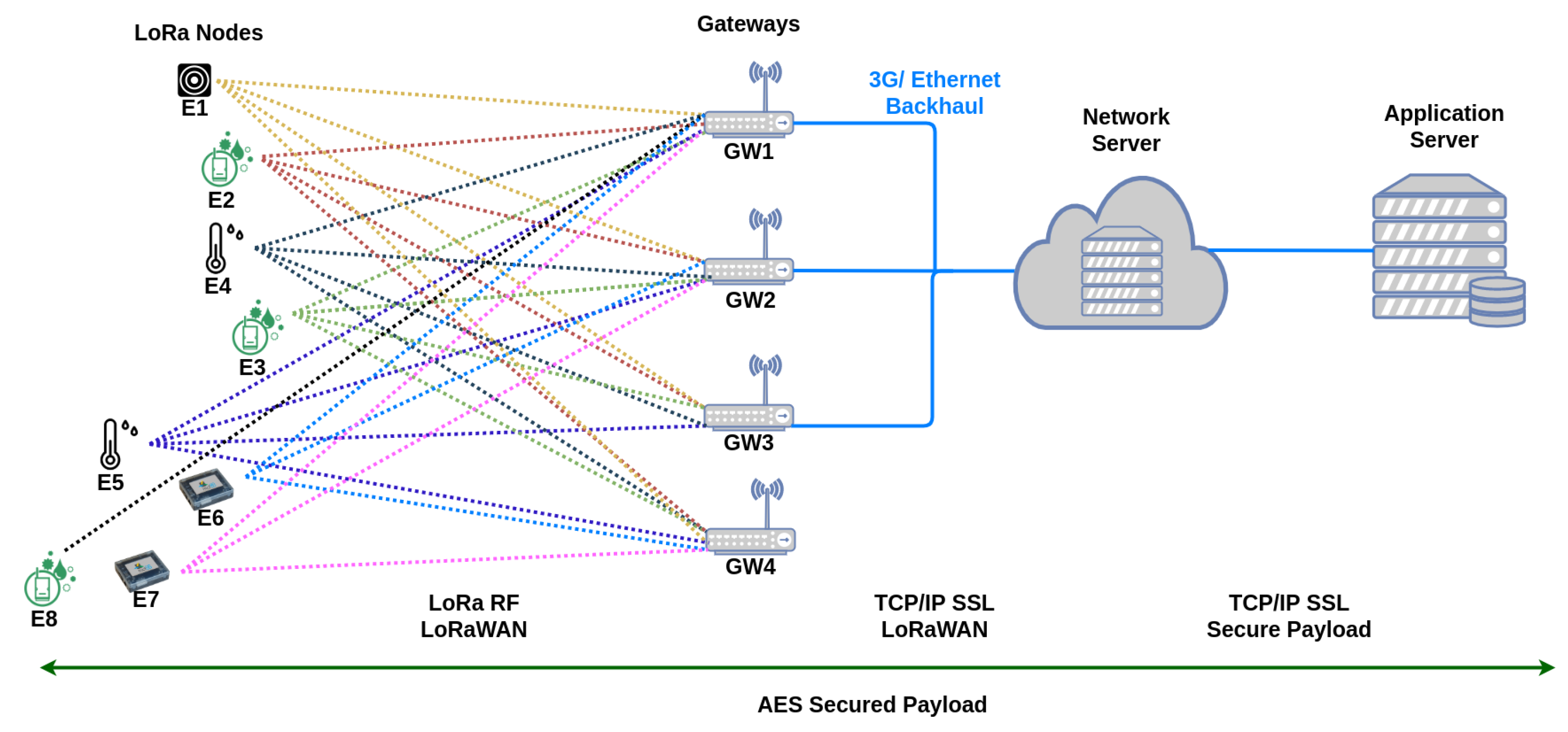
3. LoRa and LoRaWAN
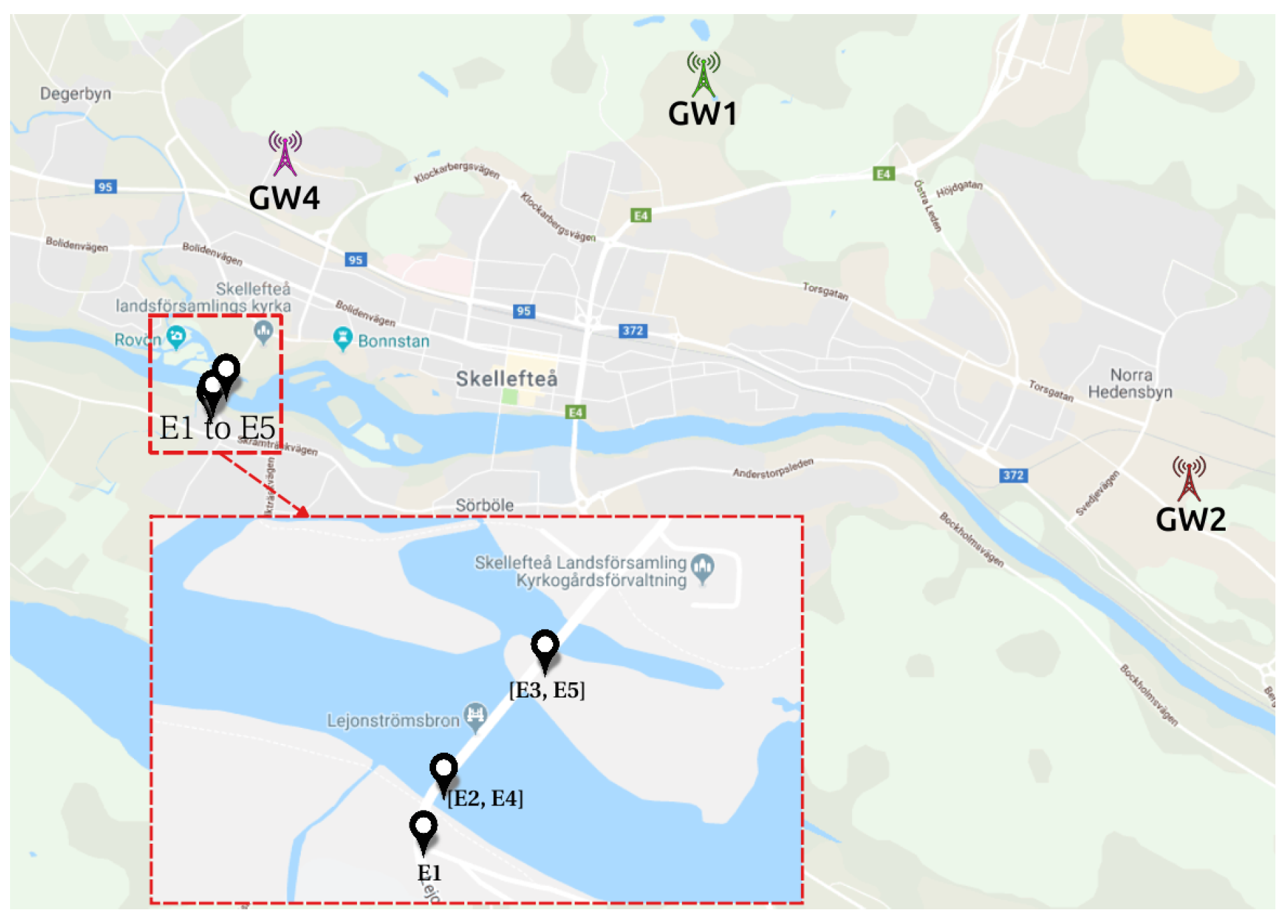
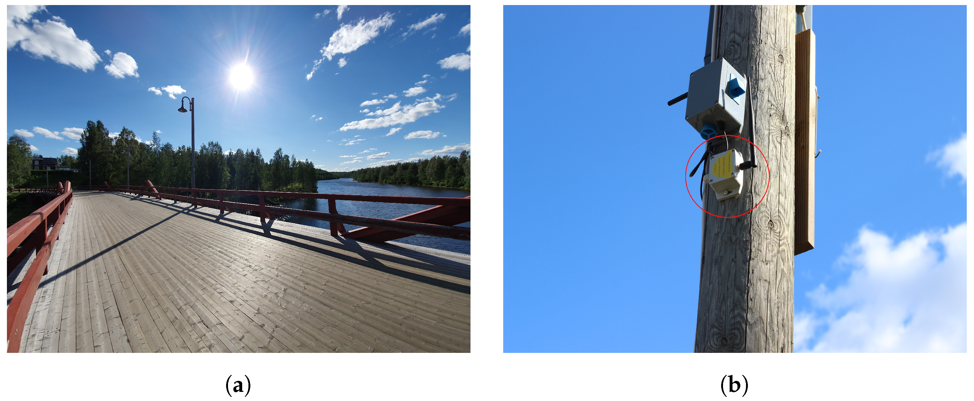
4. Experimental Setup
5. Propagation Models and Radio Planning Tool
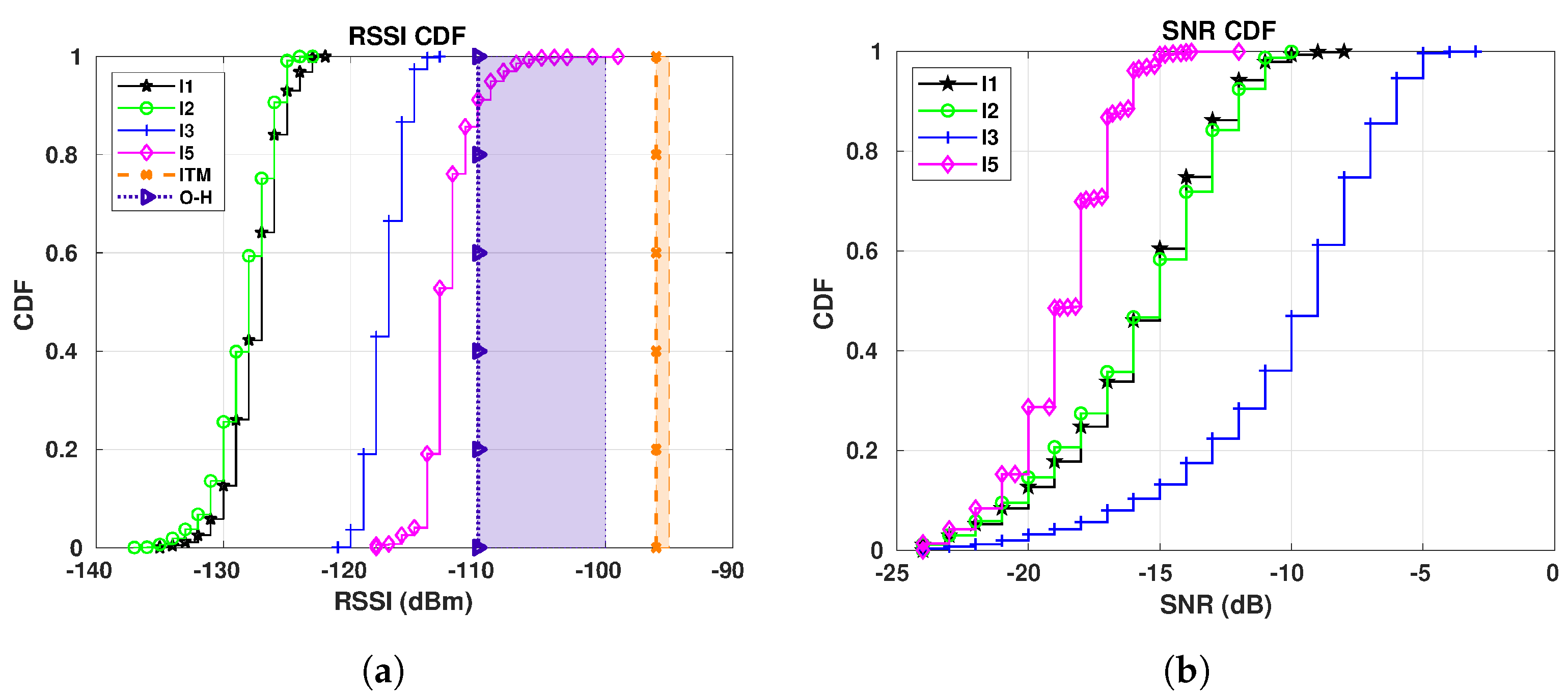
5.1. Okumura-Hata
5.2. ITM
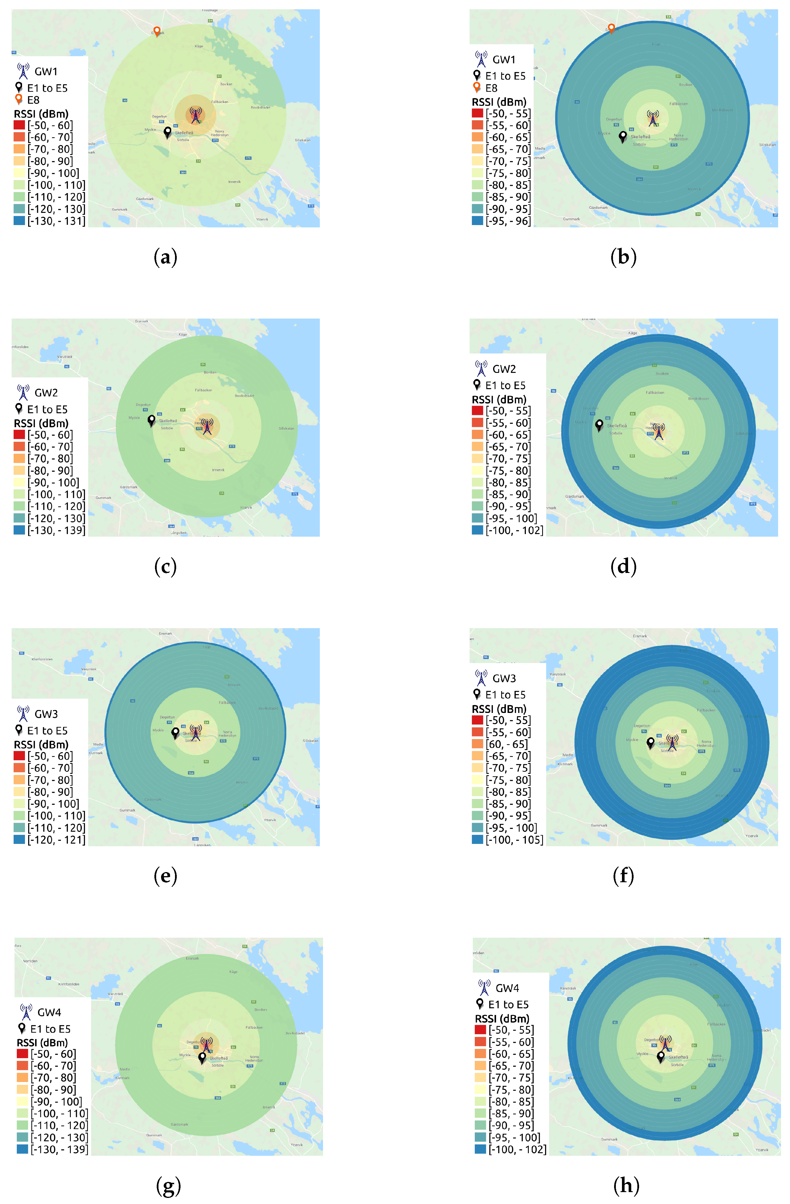
5.3. Radio Planning Tool
6. Measurement Scenarios and Evaluated Metrics
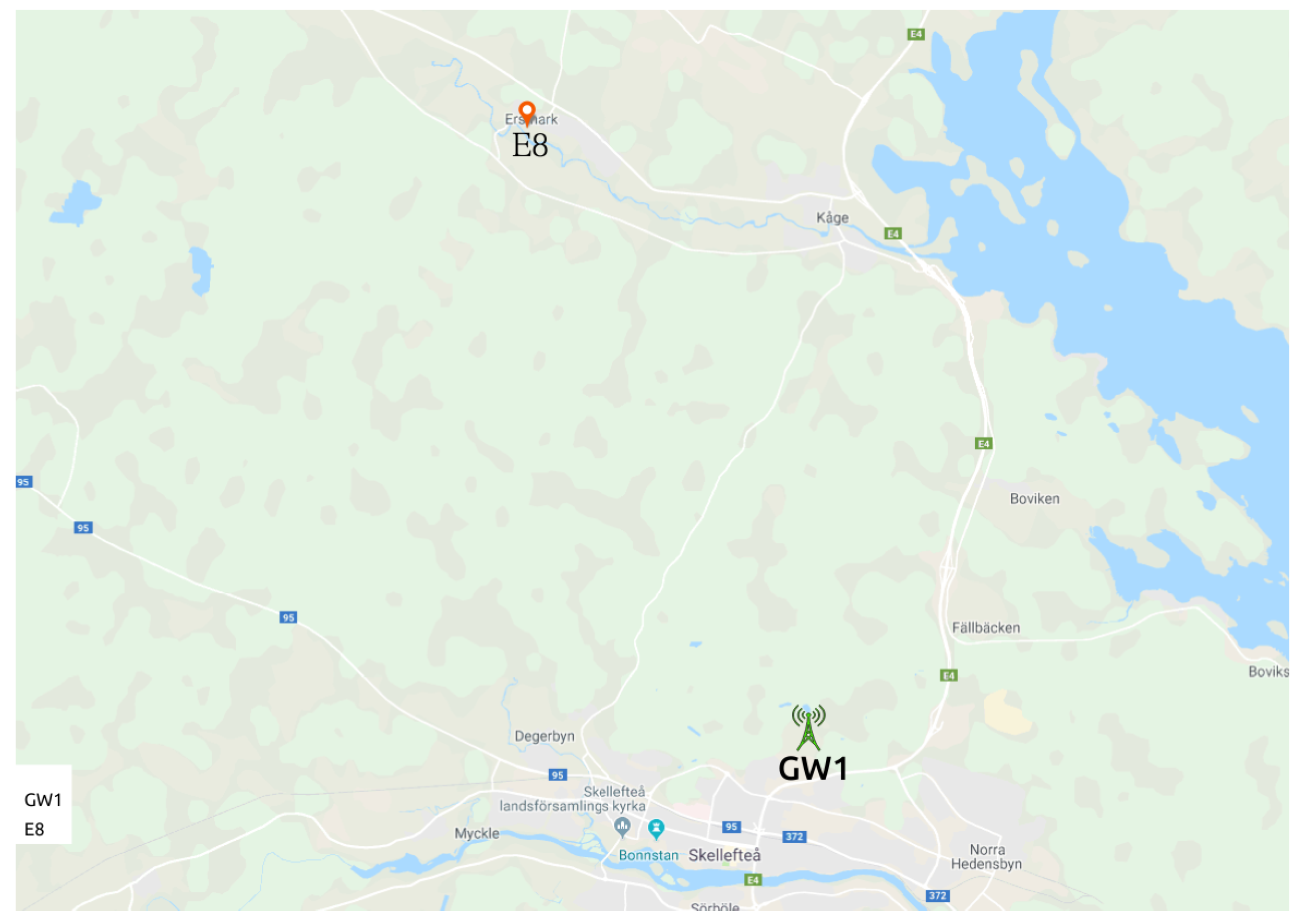
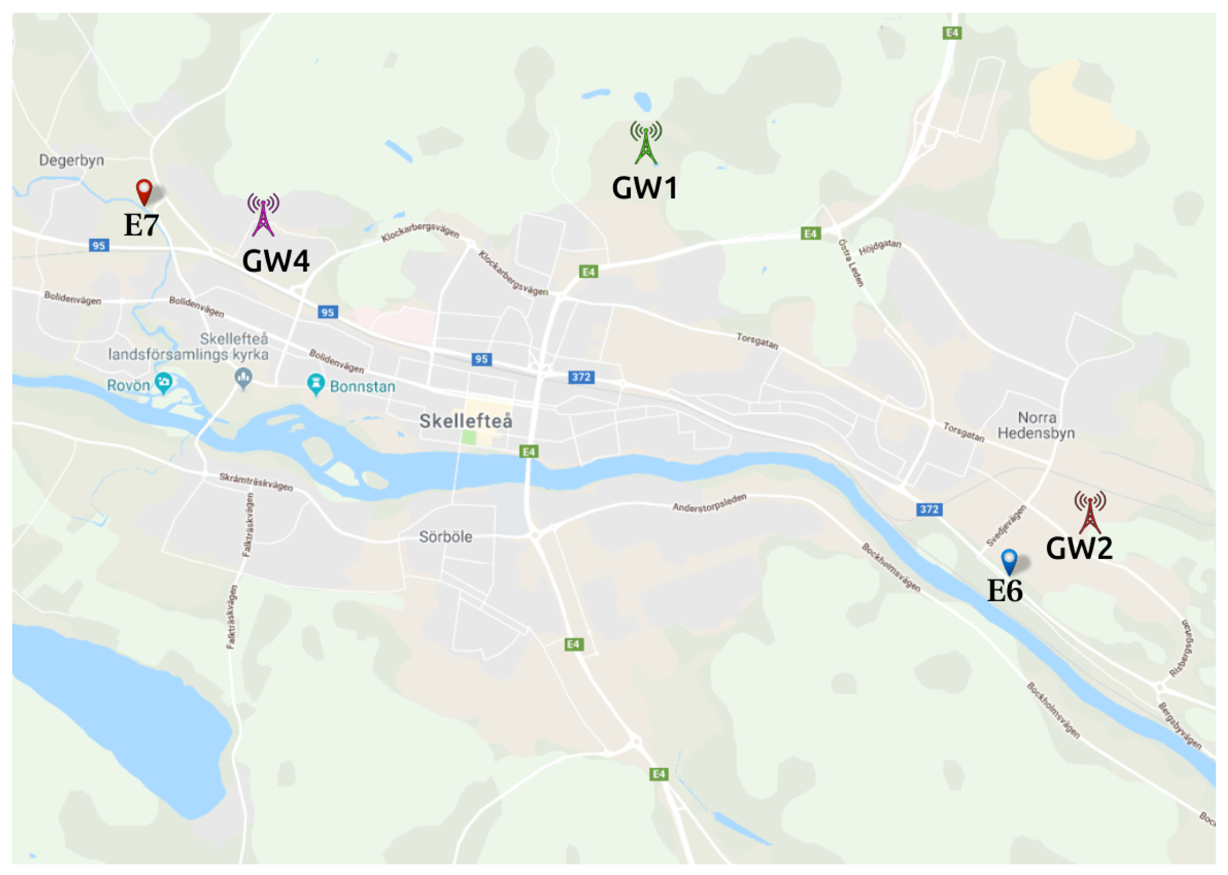
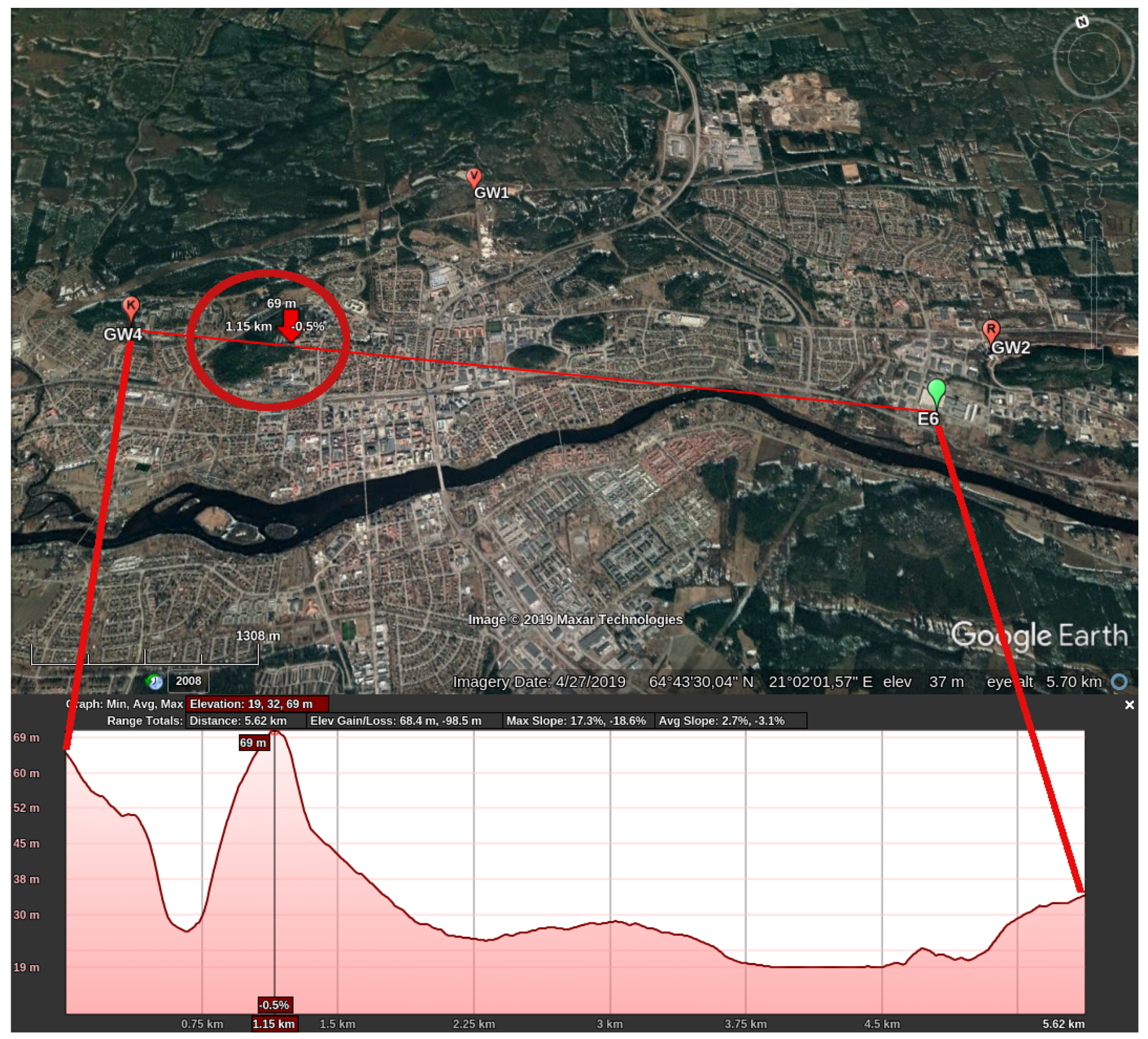
- Scenario 1 (S1): Gateway-sensor LoS link, outdoor sensors with fixed SF (sensors E1 to E5) and gateways GW1, GW2 and GW4;
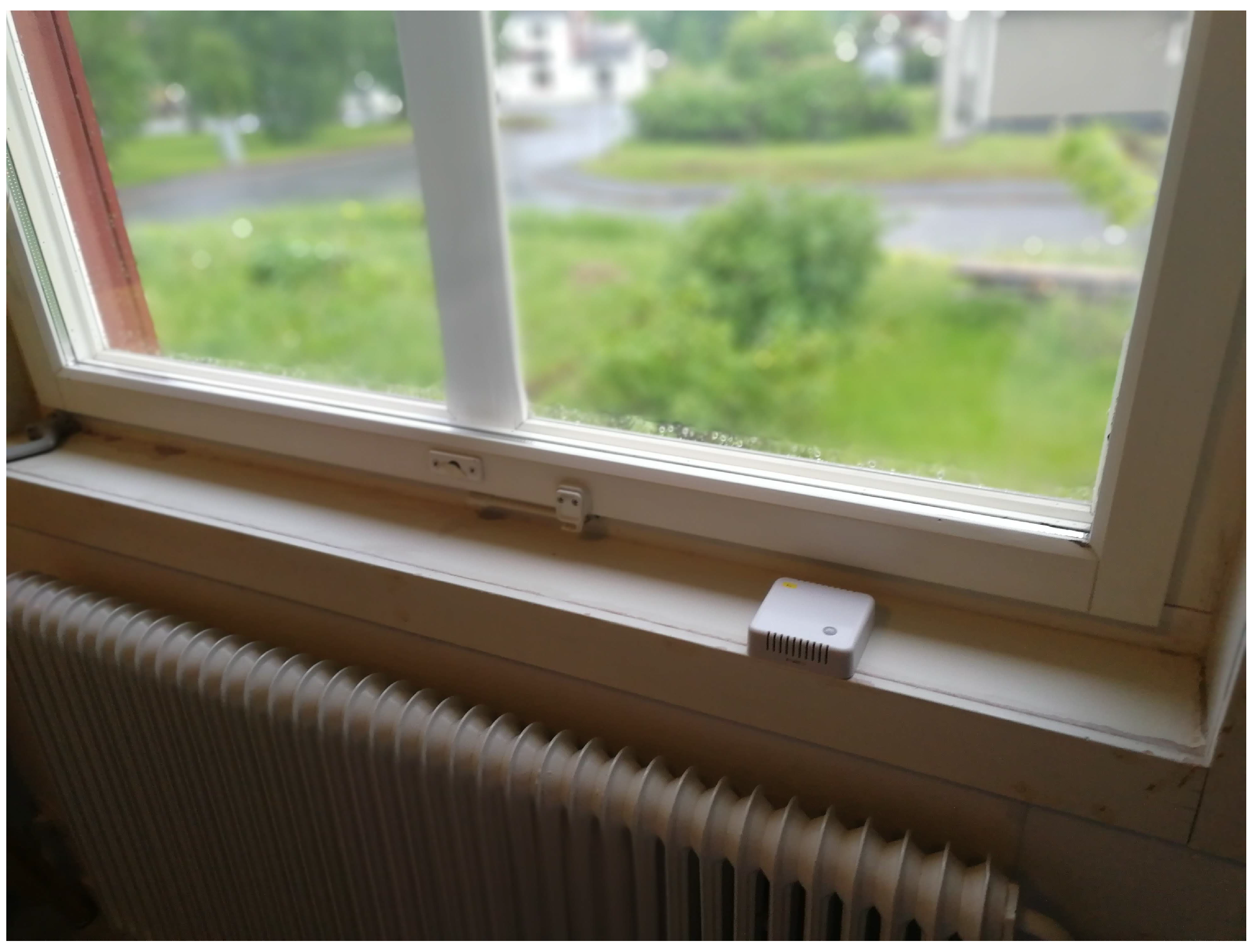
- Scenario 2 (S2): Gateway-sensor LoS link, indoor sensor with fixed SF (sensor E8) and gateways GW1, GW2 and GW4;
- Scenario 3 (S3): Gateway-sensor LoS link, outdoor sensors with ADR enabled (sensors E6 and E7) and gateways GW1, GW2 and GW4;
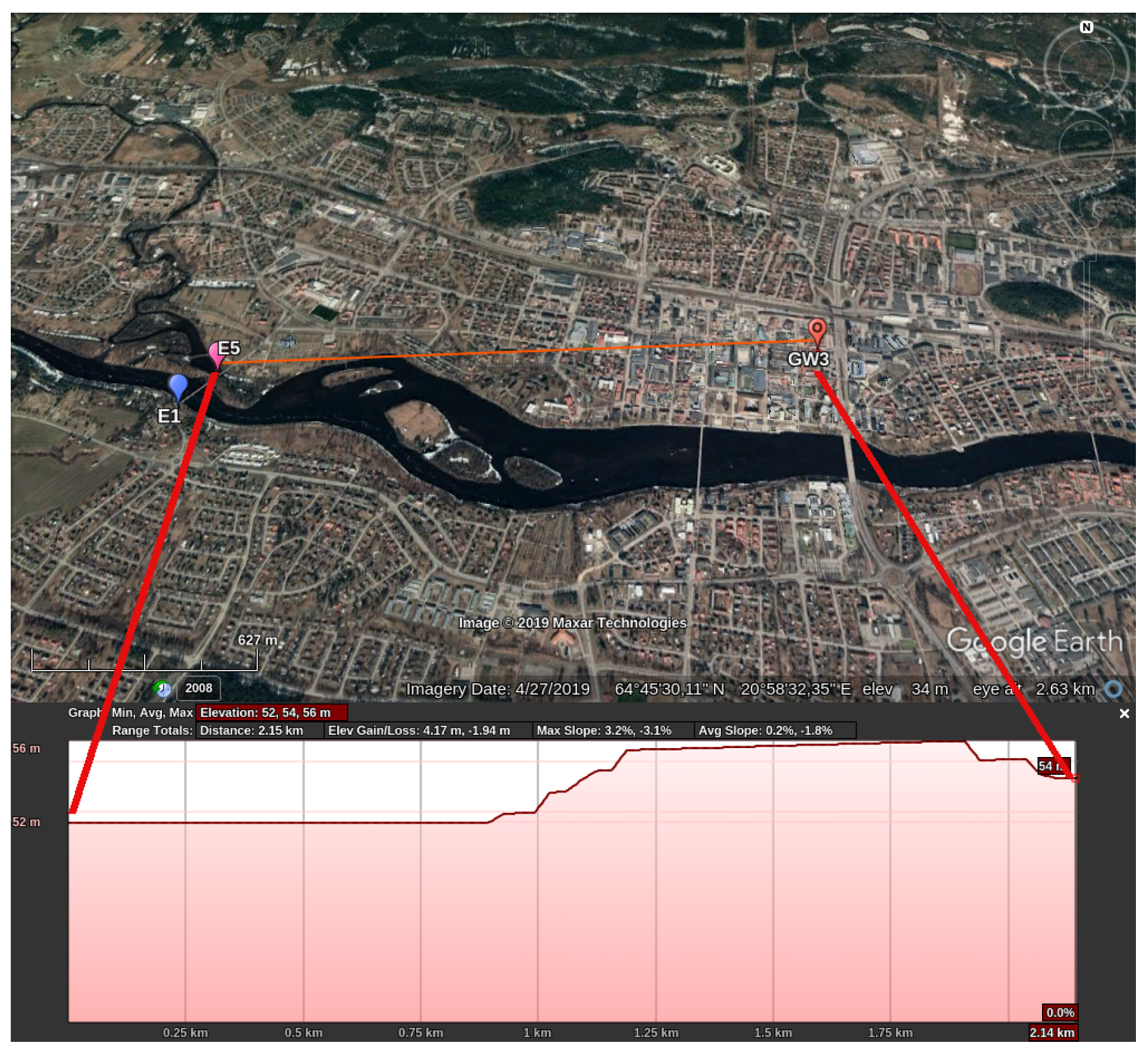
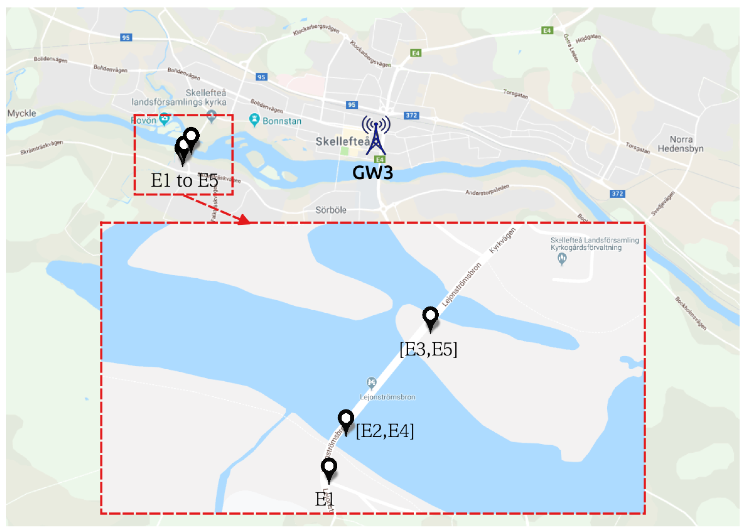
- Scenario 4 (S4): Gateway-sensor NLoS link, outdoor sensors with fixed SF (sensors E1 to E5) and gateway GW3.
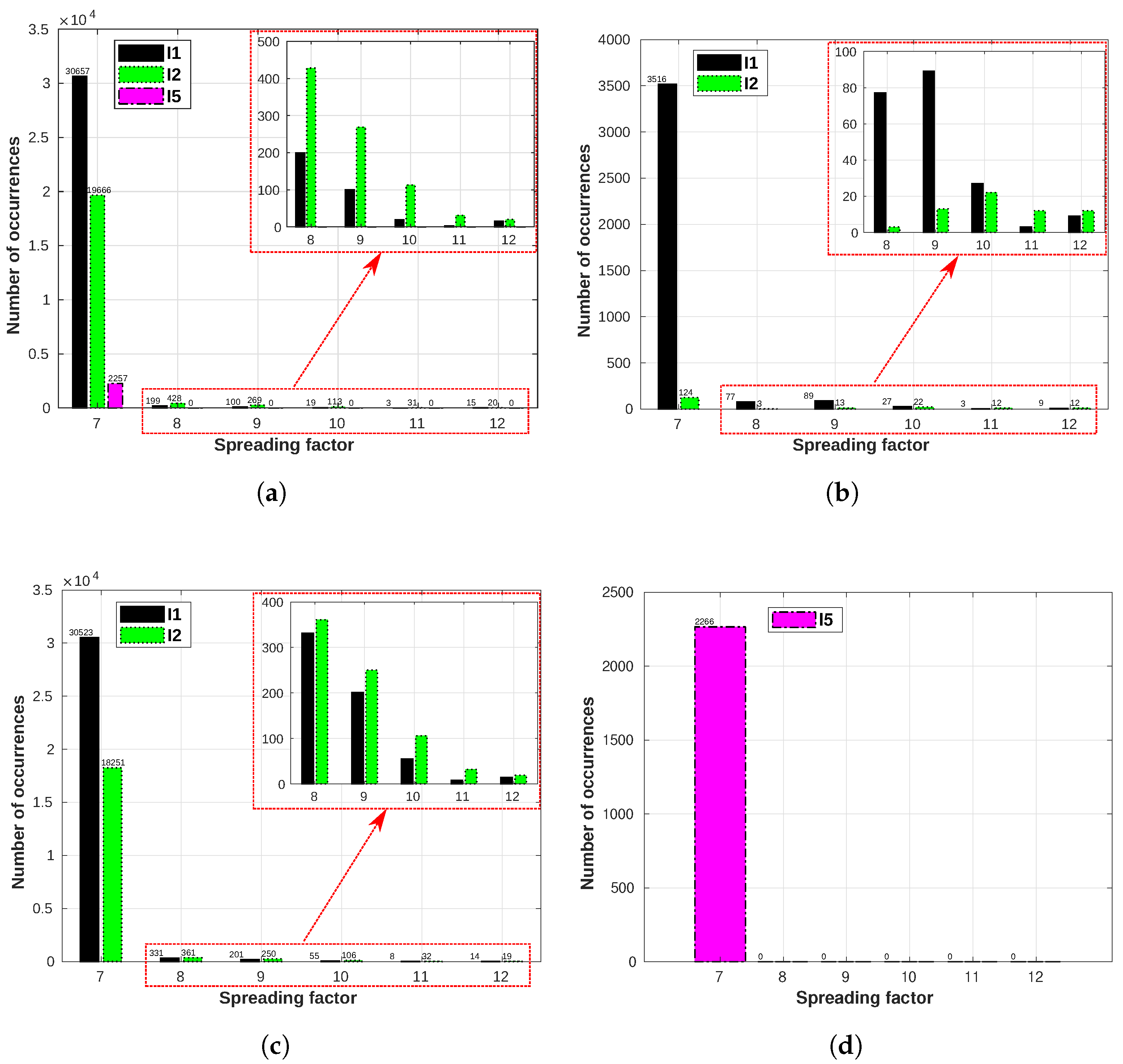
6.1. Scenario 1 (S1)—Outdoor with Fixed SF
6.2. Scenario 2 (S2)—Indoor with Fixed SF
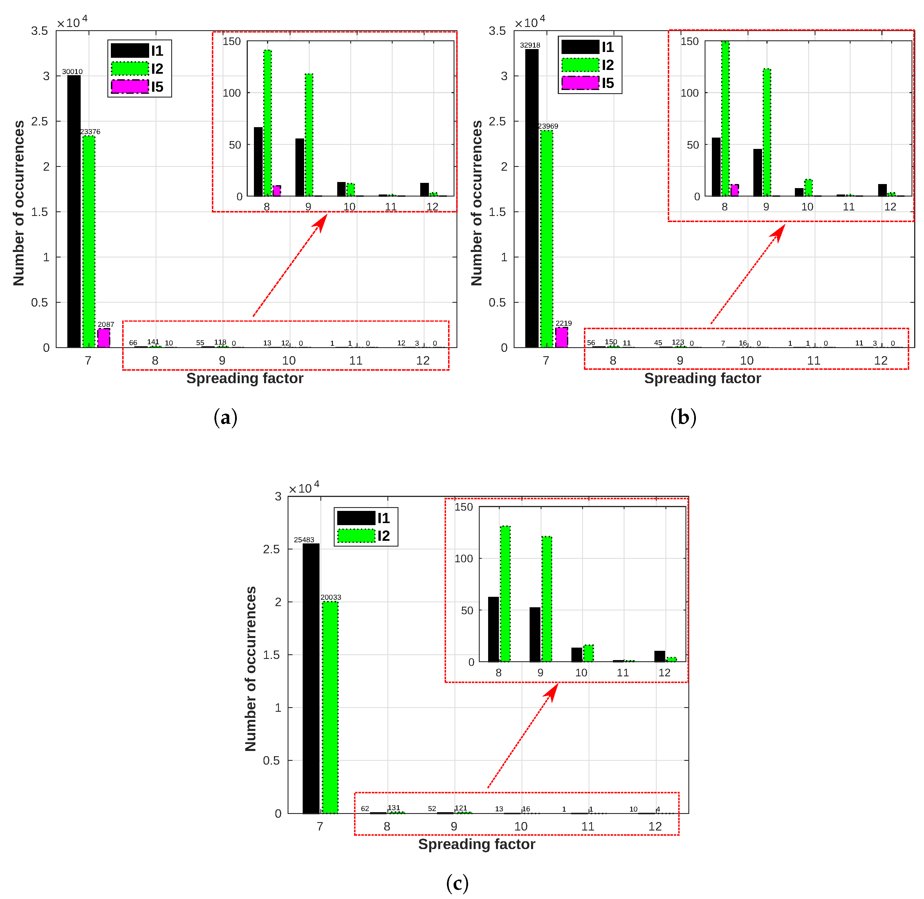
6.3. Scenario 3 (S3)—Outdoor with ADR Enabled
6.4. Scenario 4 (S4)—Gateway—Sensor NLoS Link
7. Results Presentation and Discussion
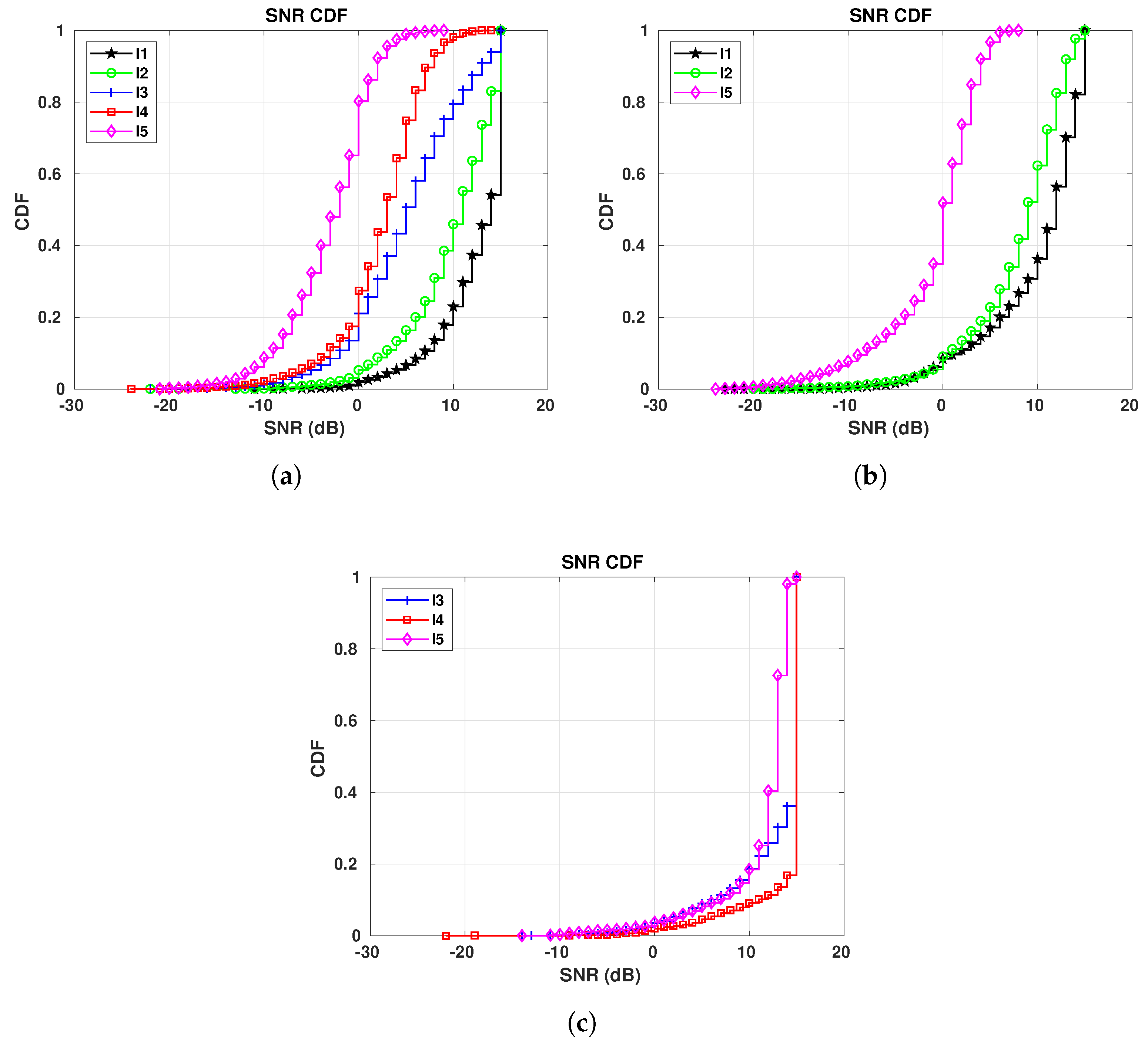
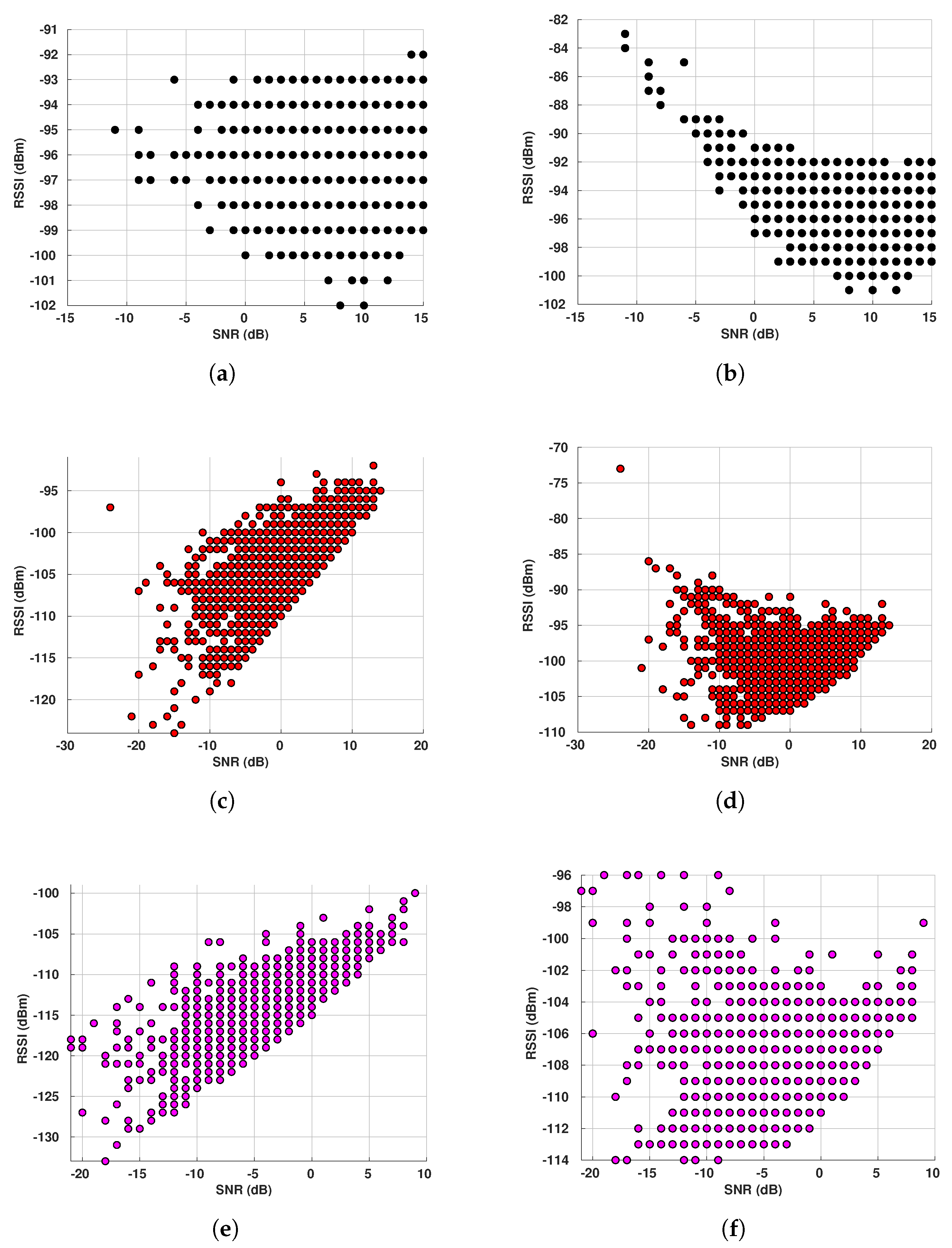
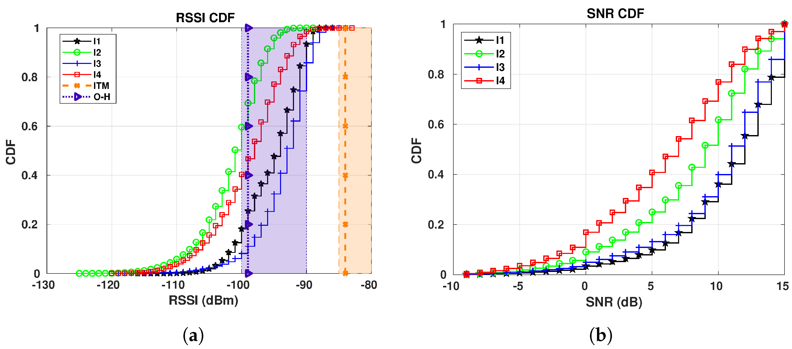
7.1. S1 Results
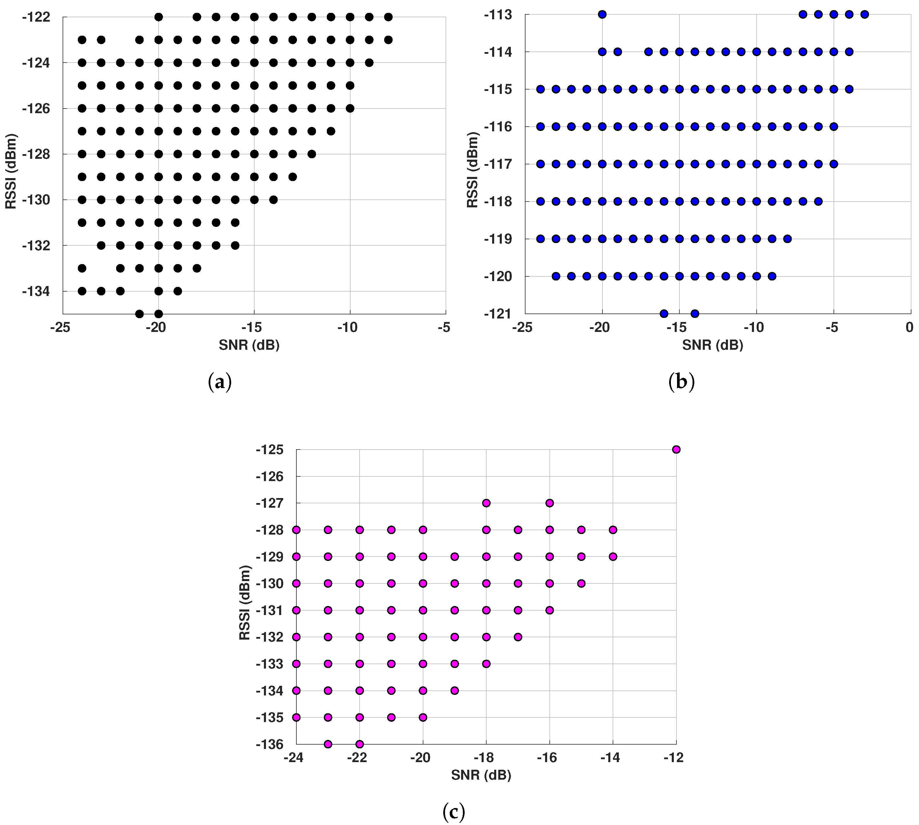
- If SNR ≥ 0: RSSIS = RSSIC = RSSI
- If SNR < 0: RSSIS = RSSIC + SNR
7.2. S2 Results
7.3. S3 Results
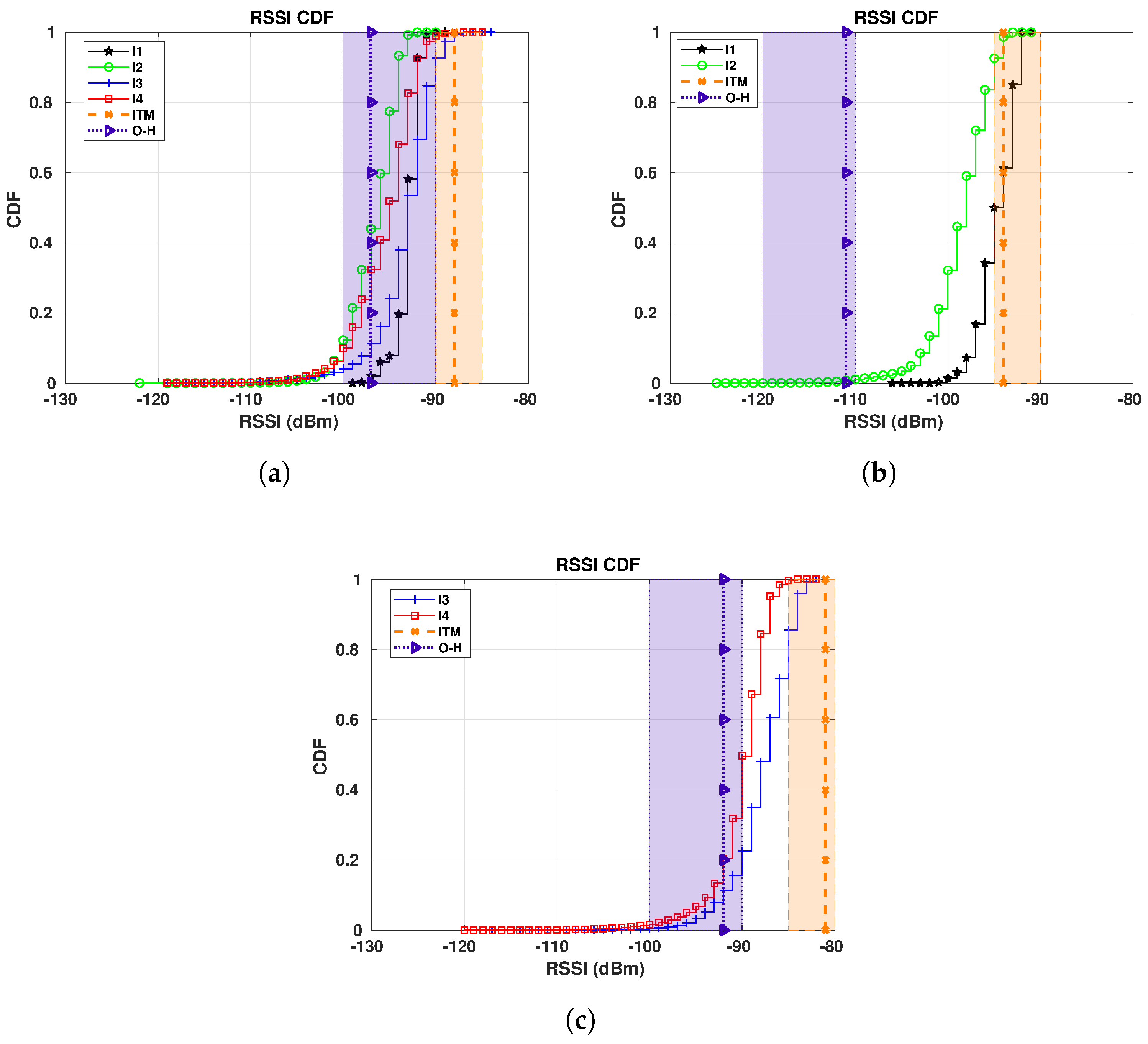
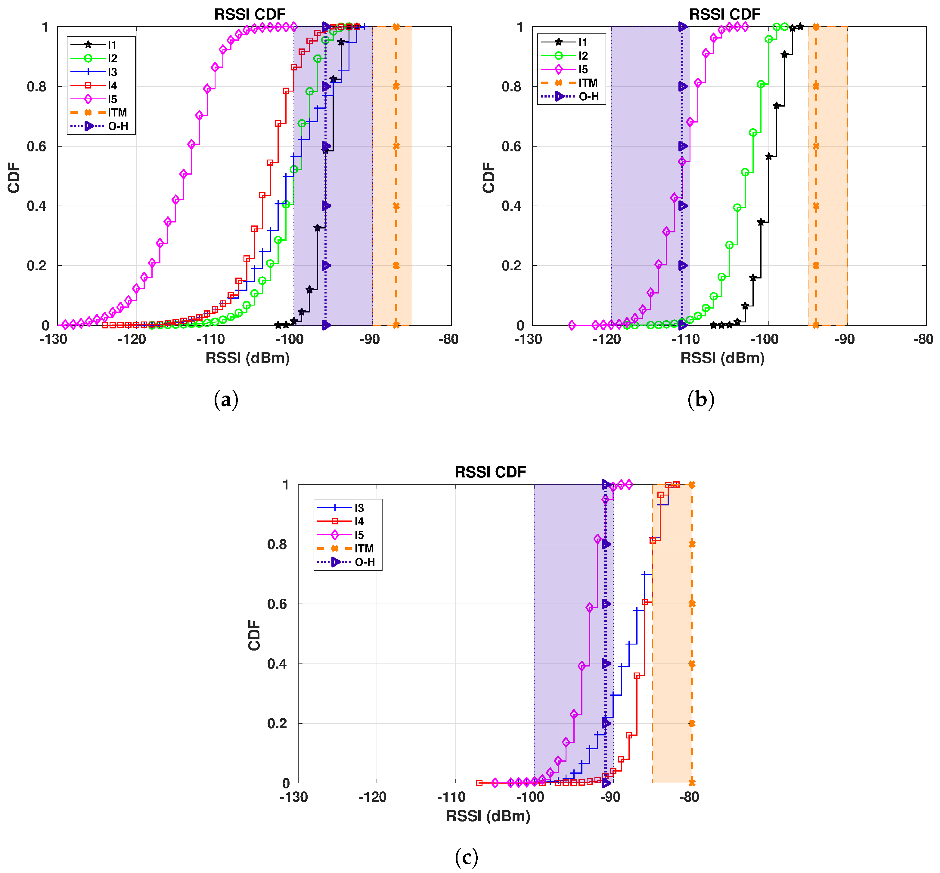
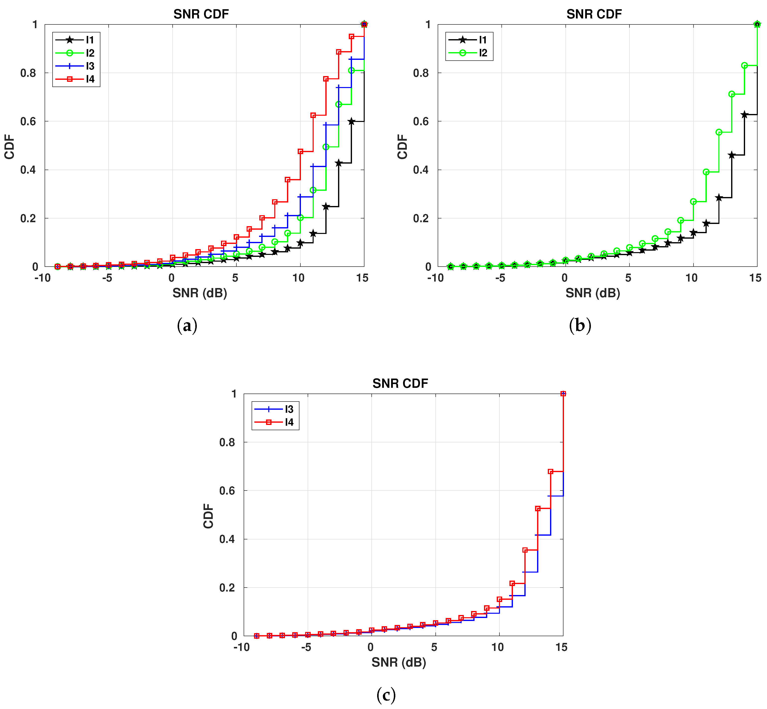
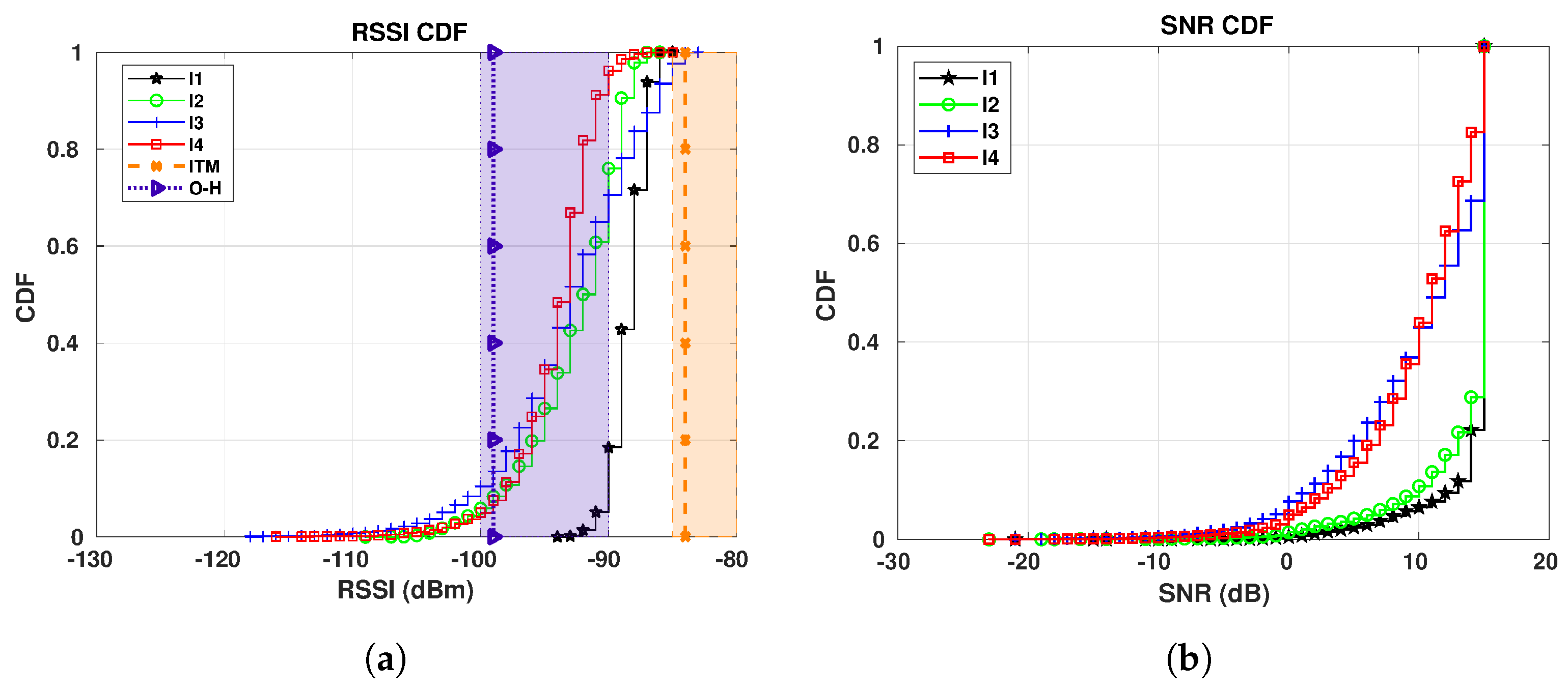
7.4. S4 Results
8. Conclusions and Lessons Learned
Author Contributions
Funding
Conflicts of Interest
Abbreviations
| ADR | Adaptive Data Rate |
| API | Application Programming Interface |
| BSF | Best Server Feature |
| BW | Bandwidth |
| CDF | Cumulative Distribution Function |
| CR | Coding Rate |
| CSS | chirp spread spectrum |
| DR | Data Rate |
| IoT | Internet of Things |
| ISM | Industrial, Scientific and Medical |
| ITM | Irregular Terrain Model |
| ITWOM | Irregular Terrain with Obstructions Model |
| LoS | Line-of-sight |
| LoRaWAN | LoRa Wide Area Network |
| LPWA | Low-Power Wide-Area |
| MAC | Medium Access Control |
| NLoS | Non-line-of-sight |
| NTIA | National Telecommunications and Information Administration |
| PHY | Physical |
| REST | Representational State Transfer |
| RF | Radio Frequency |
| RSSI | Received Signal Strength Indication |
| RSSIC | RSSI Channel |
| RSSIS | RSSI Signal |
| RTE | Radiative Transfer Engine |
| SF | Spreading Factor |
| SNR | Signal-to-Noise Ratio |
| SSiO | Societal development through Secure IoT and Open Data |
References
- What is LoRa®? Available online: https://www.semtech.com/lora/what-is-lora (accessed on 15 March 2018).
- Reynders, B.; Pollin, S. Chirp spread spectrum as a modulation technique for long range communication. In Proceedings of the 2016 Symposium on Communications and Vehicular Technologies (SCVT), Mons, Belgium, 22 November 2016; pp. 1–5. [Google Scholar] [CrossRef]
- LoRaWAN™ Specification v1.0.2. Available online: https://lora-alliance.org/resource-hub/lorawanr-specification-v102 (accessed on 1 April 2018).
- SSiO (Societal Development Through Secure IoT and Open Data). Available online: https://en.ssio.se/ (accessed on 14 August 2019).
- Molisch, A.F. Wireless Communications, 2nd ed.; Wiley Publishing: Hoboken, NJ, USA, 2011; pp. 127, 142–143. [Google Scholar]
- Irregular Terrain Model (ITM). Available online: https://www.its.bldrdoc.gov/resources/radio-propagation-software/itm/itm.aspx (accessed on 14 August 2018).
- CloudRF—Online Radio Planning. Available online: https://cloudrf.com/ (accessed on 12 June 2018).
- Haxhibeqiri, J.; De Poorter, E.; Moerman, I.; Hoebeke, J. A Survey of LoRaWAN for IoT: From Technology to Application. Sensors 2018, 18, 3995. [Google Scholar] [CrossRef] [PubMed]
- Lozano, A.; Caridad, J.; De Paz, J.F.; Villarrubia González, G.; Bajo, J. Smart Waste Collection System with Low Consumption LoRaWAN Nodes and Route Optimization. Sensors 2018, 18, 1465. [Google Scholar] [CrossRef] [PubMed]
- Johnston, S.J.; Basford, P.J.; Bulot, F.M.J.; Apetroaie-Cristea, M.; Easton, N.H.C.; Davenport, C.; Foster, G.L.; Loxham, M.; Morris, A.K.R.; Cox, S.J. City Scale Particulate Matter Monitoring Using LoRaWAN Based Air Quality IoT Devices. Sensors 2019, 19, 209. [Google Scholar] [CrossRef] [PubMed]
- Fraga-Lamas, P.; Celaya-Echarri, M.; Lopez-Iturri, P.; Castedo, L.; Azpilicueta, L.; Aguirre, E.; Suárez-Albela, M.; Falcone, F.; Fernández-Caramés, T.M. Design and Experimental Validation of a LoRaWAN Fog Computing Based Architecture for IoT Enabled Smart Campus Applications. Sensors 2019, 19, 3287. [Google Scholar] [CrossRef] [PubMed]
- Polonelli, T.; Brunelli, D.; Marzocchi, A.; Benini, L. Slotted ALOHA on LoRaWAN-Design, Analysis, and Deployment. Sensors 2019, 19, 838. [Google Scholar] [CrossRef] [PubMed]
- Kim, S.; Yoo, Y. Contention-Aware Adaptive Data Rate for Throughput Optimization in LoRaWAN. Sensors 2018, 18, 1716. [Google Scholar] [CrossRef] [PubMed]
- Parri, L.; Parrino, S.; Peruzzi, G.; Pozzebon, A. Low Power Wide Area Networks (LPWAN) at Sea: Performance Analysis of Offshore Data Transmission by Means of LoRaWAN Connectivity for Marine Monitoring Applications. Sensors 2019, 19, 3239. [Google Scholar] [CrossRef] [PubMed]
- Petrić, T.; Goessens, M.; Nuaymi, L.; Toutain, L.; Pelov, A. Measurements, performance and analysis of LoRa FABIAN, a real-world implementation of LPWAN. In Proceedings of the 2016 IEEE 27th Annual International Symposium on Personal, Indoor, and Mobile Radio Communications (PIMRC), Valencia, Spain, 4–7 September 2016; pp. 1–7. [Google Scholar] [CrossRef]
- Georgiou, O.; Raza, U. Low Power Wide Area Network Analysis: Can LoRa Scale? IEEE Wirel. Commun. Lett. 2017, 6, 162–165. [Google Scholar] [CrossRef]
- Petäjäjärvi, J.; Mikhaylov, K.; Roivainen, A.; Hanninen, T.; Pettissalo, M. On the coverage of LPWANs: Range evaluation and channel attenuation model for LoRa technology. In Proceedings of the 2015 14th International Conference on ITS Telecommunications (ITST), Copenhagen, Denmark, 2–4 December 2015; pp. 55–59. [Google Scholar] [CrossRef]
- Sanchez-Iborra, R.; Sanchez-Gomez, J.; Ballesta-Viñas, J.; Cano, M.D.; Skarmeta, A.F. Performance Evaluation of LoRa Considering Scenario Conditions. Sensors 2018, 18, 772. [Google Scholar] [CrossRef] [PubMed]
- Harinda, E.; Hosseinzadeh, S.; Larijani, H.; Gibson, R.M. Comparative Performance Analysis of Empirical Propagation Models for LoRaWAN 868MHz in an Urban Scenario. In Proceedings of the 2019 IEEE 5th World Forum on Internet of Things (WF-IoT’19), Limerick, Ireland, 15–18 April 2019; IEEE: Piscataway, NJ, USA, 2019; pp. 154–159. [Google Scholar] [CrossRef]
- Bezerra, N.S.; Åhlund, C.; Saguna, S.; de Sousa, V.A. Propagation Model Evaluation for LoRaWAN: Planning Tool Versus Real Case Scenario. In Proceedings of the 2019 IEEE 5th World Forum on Internet of Things (WF-IoT), Limerick, Ireland, 15–18 April 2019; pp. 1–6. [Google Scholar] [CrossRef]
- Shumate, S.E. Deterministic Equations for Computer Approximation of ITU-R P.1546-2. In Proceedings of the International Symposium on Advanced Radio Technologies and The Working Party Meetings for ITU-R WP3J, 3K, 3L and 3M hosted by National Institute of Standards and Technology, Boulder, CO, USA, 2–4 June 2008. [Google Scholar] [CrossRef]
- Shumate, S.E. Longley-Rice and ITU-P.1546 Combined: A New International Terrain-Specific Propagation Model. In Proceedings of the 2010 IEEE 72nd Vehicular Technology Conference—Fall, Ottawa, ON, Canada, 6–9 September 2010; pp. 1–5. [Google Scholar] [CrossRef]
- Cattani, M.; Boano, C.A.; Römer, K. An Experimental Evaluation of the Reliability of LoRa Long-Range Low-Power Wireless Communication. J. Sens. Actuator Netw. 2017, 6, 7. [Google Scholar] [CrossRef]
- Gaelens, J.; Van Torre, P.; Verhaevert, J.; Rogier, H. LoRa Mobile-To-Base-Station Channel Characterization in the Antarctic. Sensors 2017, 17, 1903. [Google Scholar] [CrossRef] [PubMed]
- Boano, C.A.; Cattani, M.; Römer, K. Impact of Temperature Variations on the Reliability of LoRa—An Experimental Evaluation. In Proceedings of the 7th International Conference on Sensor Networks—Volume 1: SENSORNETS, Funchal, Portugal, 22–24 January 2018; INSTICC, SciTePress: Setúbal, Portugal, 2018; pp. 39–50. [Google Scholar] [CrossRef]
- Iova, O.; Murphy, A.L.; Picco, G.P.; Ghiro, L.; Molteni, D.; Ossi, F.; Cagnacci, F. LoRa from the City to the Mountains: Exploration of Hardware and Environmental Factors. In Proceedings of the 2017 International Conference on Embedded Wireless Systems and Networks (EWSN 2017), Uppsala, Sweden, 20–22 February 2017; Junction Publishing: Chelsea, VT, USA, 2017; pp. 317–322. [Google Scholar]
- What is LoRaWAN™ Specification? Available online: https://lora-alliance.org/about-lorawan (accessed on 15 March 2018).
- Semtech. Available online: https://www.semtech.com/ (accessed on 13 April 2019).
- AN1200.22—LoRa™ Modulation Basics. Available online: https://www.semtech.com/uploads/documents/an1200.22.pdf (accessed on 23 November 2018).
- Petäjäjärvi, J.; Mikhaylov, K.; Pettissalo, M.; Janhunen, J.; Iinatti, J. Performance of a low-power wide-area network based on LoRa technology: Doppler robustness, scalability, and coverage. Int. J. Distrib. Sens. Netw. 2017, 13. [Google Scholar] [CrossRef]
- LoRaWAN™ Regional Parameters v1.0.2rB. Available online: https://lora-alliance.org/sites/default/files/2018-05/lorawan_regional_parameters_v1.0.2_final_1944_1.pdf (accessed on 15 March 2019).
- What is LoRaWAN™? Available online: https://lora-alliance.org/resource-hub/what-lorawanr (accessed on 19 September 2019).
- Wirnet IBTS. Available online: https://www.kerlink.com/product/wirnet-ibts/ (accessed on 12 September 2018).
- Network Operations. Available online: https://www.kerlink.com/iot-solutions-services/network-operations/ (accessed on 12 March 2018).
- LoRa® ELT-1/ ELT-2-HP. Available online: https://www.elsys.se/en/elt-1/ (accessed on 12 March 2018).
- LoRa®ERS. Available online: https://www.elsys.se/en/ers/ (accessed on 12 March 2018).
- MCF-LW06485. Available online: https://www.mcf88.it/prodotto/mcf-lw06485/ (accessed on 3 April 2019).
- Massé, M. REST API Design Rulebook, 1st ed.; O’Reilly Media: Newton, MA, USA, 2011; pp. 5–6. [Google Scholar]
- Phillips, C.; Sicker, D.; Grunwald, D. A Survey of Wireless Path Loss Prediction and Coverage Mapping Methods. IEEE Commun. Surv. Tutor. 2013, 15, 255–270. [Google Scholar] [CrossRef]
- CloudRF Web Interface Documentation. Available online: https://cloudrf.com/web_docs (accessed on 12 May 2019).
- Google Maps. Available online: https://www.google.com/maps (accessed on 17 May 2019).
- Balderväder—Statistik. Available online: http://balderskolan.se/vader/stat.php (accessed on 30 May 2019).
- Sara Culture House. Available online: https://vaxer.skelleftea.se/project/sarakulturhus/# (accessed on 26 August 2019).
- Strömsör Living Area. Available online: https://vaxer.skelleftea.se/project/stromsor-2/ (accessed on 26 August 2019).
- Google Earth. Available online: https://earth.google.com/web/ (accessed on 13 July 2019).
- District Heating. Available online: https://www.energimyndigheten.se/en/sustainability/households/heating-your-home/district-heating/ (accessed on 27 August 2019).
- Anjum, M.; Khan, M.A.; Ali Hassan, S.; Mahmood, A.; Gidlund, M. Analysis of RSSI Fingerprinting in LoRa Networks. In Proceedings of the 2019 15th International Wireless Communications Mobile Computing Conference (IWCMC), Tangier, Morocco, 24–28 June 2019; pp. 1178–1183. [Google Scholar] [CrossRef]
- Friis, H.T. Noise Figures of Radio Receivers. Proc. IRE 1944, 32, 419–422. [Google Scholar] [CrossRef]
- Ghasemi, A.; Abedi, A.; Ghasemi, F. Propagation Engineering in Wireless Communications, 1st ed.; Springer: New York, NY, USA, 2012; p. 202. [Google Scholar]
- Semtech. SX1276/77/78/79—137 MHz to 1020 MHz Low Power Long Range Transceiver; Rev. 6; Semtech: Camarillo, CA, USA, 2019. [Google Scholar]
- Rappaport, T.S. Wireless Communications: Principles and Practice, 2nd ed.; Prentice Hall: Upper Saddle River, NJ, USA, 2001; p. 72. [Google Scholar]
- ITU. P.530-17: Propagation Data and Prediction Methods Required for the Design of Terrestrial Line-of-Sight Systems; Recommendation P.530-17; International Telecommunication Union: Geneva, Switzerland, 2017. [Google Scholar]
- ITU. P.840-7: Attenuation Due to Clouds and Fog; Recommendation P.840-7; International Telecommunication Union: Geneva, Switzerland, 2017. [Google Scholar]
- Snow Depths Chart for the City of Skellefteå. Available online: http://balderskolan.se/vader/snodjupdiagram.htm (accessed on 14 July 2019).
- In-Depth Study of the General Plan for Skellefteå Municipality. Available online: https://www.skelleftea.se/Bygg%20och%20miljokontoret/Innehallssidor/Bifogat/Skelleftedalen_F%C3%B6ruts%C3%A4ttningar.pdf (accessed on 17 July 2019).
- Chulsung, P.; Lahiri, K.; Raghunathan, A. Battery discharge characteristics of wireless sensor nodes: An experimental analysis. In Proceedings of the 2005 Second Annual IEEE Communications Society Conference on Sensor and Ad Hoc Communications and Networks (IEEE SECON 2005), Santa Clara, CA, USA, 26–29 September 2005; pp. 430–440. [Google Scholar] [CrossRef]
- ITU. P.676-10: Attenuation by Atmospheric Gases; Recommendation P.676-10; International Telecommunication Union: Geneva, Switzerland, 2013. [Google Scholar]


| Data Rate | Configuration | Indicative Physical Bit Rate (bits/s) |
|---|---|---|
| 0 | LoRa: SF12/125 kHz | 250 |
| 1 | LoRa: SF11/125 kHz | 440 |
| 2 | LoRa: SF10/125 kHz | 980 |
| 3 | LoRa: SF9/125 kHz | 1760 |
| 4 | LoRa: SF8/125 kHz | 3125 |
| 5 | LoRa: SF7/125 kHz | 5470 |
| Gateway | Altitude (m) | Lat, Long |
|---|---|---|
| GW1 | 165 | 64.76736, 20.97684 |
| GW2 | 76 | 64.74462, 21.04086 |
| GW3 | 54 | 64.75089, 20.95882 |
| GW4 | 66 | 64.76292, 20.92167 |
| Sensor | Model | Measurements Capabilities | Spreading Factor | Reporting Interval | Coding Rate | Lat, Long |
|---|---|---|---|---|---|---|
| E1 | Elsys ELT-1 | Temperature, humidity, and orientation | 7 | 1 min | 4/5 | 64.748983, 20.912189 |
| E2 | Elsys ELT-1 | Temperature, humidity, and orientation | 10 | 5 min | 4/5 | 64.749404, 20.912538 |
| E3 | Elsys ELT-1 | Temperature, humidity, and orientation | 10 | 3 min | 4/5 | 64.750306, 20.914273 |
| E4 | Elsys ELT-1 | Temperature, humidity, and orientation | 12 | 3 min | 4/5 | 64.749404, 20.912538 |
| E5 | Elsys ELT-1 | Temperature, humidity, and orientation | 12 | 5 min | 4/5 | 64.750306, 20.914273 |
| E6 | mcf88 MCF-LW06485 | Tilt (accelerometer), temperature, current, voltage, and sound | ADR | 5 min | 4/5 | 64.742171, 21.029322 |
| E7 | mcf88 MCF-LW06485 | Tilt (accelerometer), temperature, current, voltage, and sound | ADR | 5 min | 4/5 | 64.764916, 20.904624 |
| E8 | Elsys ERS | Temperature, humidity, light, and motion | 12 | 5 min | 4/5 | 64.849365, 20.889126 |
| Transmitter (Gateway) | Antenna (Gateway) | Receiver (Sensors) | CloudRF Output | ||||
|---|---|---|---|---|---|---|---|
| Frequency | 868 MHz | Type | OEM Half-Wave Dipole | Height(s) AGL | 2 m | Terrain resolution | 10 m/ 33 ft |
| Polarization | Vertical | Antenna Gain | 3 dBi | ||||
| Gateway RF Power | 20 dBm | Direction | 0 | Antenna Gain | 3 dBi | Colour scheme | Greyscale GIS |
| Tilt | 0 | Units of measurement | Received Power (dBm) | ||||
| Lat, long and height | From Table 2 | Tx Gain | 3 dBi | Units of measurement | Received Power (dBm) | Radius | 10 km |
| Feeder loss | 0 dB 1 dB | Sensitivity | −140 dBm | ||||
| Model | |||
|---|---|---|---|
| ITM | Okumura-Hata (O-H) | ||
| Reliability | 90.00% | Environment | All gateways: Average |
| Terrain conductivity | GW1: Mountain/Sand | Knife-edge diffraction | off |
| GW2 to GW4: City | |||
| Radio climate | Maritime temperate (land) | Random clutter | 0 m |
| Random clutter | 0 m | Point clutter | off |
| Point clutter | off | ||
| Propagation Model | |||||
|---|---|---|---|---|---|
| ITM | Okumura-Hata | ||||
| Sensor | Gateway | RSSI(dBm) | Sensor | Gateway | RSSI(dBm) |
| E1 | GW1 | −88 | E1 | GW1 | −97 |
| GW2 | −94 | GW2 | −111 | ||
| GW3 | −84 | GW3 | −99 | ||
| GW4 | −81 | GW4 | −92 | ||
| E5 | GW1 | −87 | E5 | GW1 | −96 |
| GW2 | −94 | GW2 | −111 | ||
| GW3 | −84 | GW3 | −99 | ||
| GW4 | −80 | GW4 | −91 | ||
| E8 | GW1 | −96 | E8 | GW1 | −110 |
| Label | Temperature Average (°C) | Minimum Temperature (°C) | Maximum Temperature (°C) | Time Period | Equipment in Operation |
|---|---|---|---|---|---|
| I1 | −16.96 | −28.7 | −6.9 | 16/01/2019–07/02/2019 | GW1, GW2 and GW3 E1 to E8 |
| I2 | −9.45 | −17.8 | 4.5 | 22/12/2018–06/01/2019 | GW1, GW2 and GW3 E1 to E8 |
| I3 | −0.15 | −11.4 | 7.8 | 25/10/2018–04/11/2018 | GW1, GW3 and GW4 E1 to E5; E8 |
| I4 | 6.56 | −3.5 | 20.8 | 30/09/2018–14/10/2018 | GW1, GW3 and GW4 E1 to E5 |
| I5 | 13.22 | 3.2 | 24.8 | 15/05/2019–22/05/2019 | GW1, GW2 and GW4 E2 to E8 |
| Scenario | Gateways/ Sensors | Measurement Periods | Evaluation Metrics | Assessment Targets |
|---|---|---|---|---|
| S1 | GW1, GW2, GW4 E1 to E5 | I1 to I5 | RSSI and SNR | Measured RSSI CDF vs CloudRF estimations per period Comparison of SNR CDFs per period RSSI vs SNR per period |
| S2 | GW1, GW2, GW4 E8 | I1, I2, I3, and I5 | RSSI and SNR | Measured RSSI CDF vs CloudRF estimations per period Comparison of SNR CDFs per period RSSI vs SNR per period |
| S3 | GW1, GW2, GW4 E6 and E7 | I1, I2 and I5 | SF histogram | ADR behavior per period |
| S4 | GW3 E1 to E5 | I1 to I4 | RSSI and SNR SF histogram | Measured RSSI CDF vs CloudRF estimations per period Comparison of SNR CDFs per period |
| Gateway | Map Range Estimation (dBm) | Best Server Feature (BSF) Estimation (dBm) | Main Conclusions |
|---|---|---|---|
| GW1 | O-H: −100 to −90 ITM: −90 to −85 | O-H: −95 ITM: −87 | O-H: less than 50% of data is within the estimated range ITM: CDF curves are out of the estimated range ITM: estimation by the BSF does not cross any CDF ITM overestimated the RSSI values |
| GW2 | O-H: −120 to −110 ITM: −95 to −90 | O-H: −111 ITM: −94 | O-H: very small parts of I2 is within the range O-H: 65% of I5 is within the range Neither ITM nor H-O fits I1 ITM overestimated the RSSI values |
| GW4 | O-H: −100 to −90 ITM: −85 to −80 | O-H: −91 ITM: −80 | O-H: most of the data for I5 is within the range O-H: small parts of I3 and I4 are within the range O-H: estimation by the BSF crosses all the CDFs ITM: estimation by the BSF does not cross any CDF ITM: only parts of I3, I4 and I5 are within the range ITM overestimated the RSSI values |
© 2019 by the authors. Licensee MDPI, Basel, Switzerland. This article is an open access article distributed under the terms and conditions of the Creative Commons Attribution (CC BY) license (http://creativecommons.org/licenses/by/4.0/).
Share and Cite
Souza Bezerra, N.; Åhlund, C.; Saguna, S.; de Sousa, V.A. Temperature Impact in LoRaWAN—A Case Study in Northern Sweden. Sensors 2019, 19, 4414. https://doi.org/10.3390/s19204414
Souza Bezerra N, Åhlund C, Saguna S, de Sousa VA. Temperature Impact in LoRaWAN—A Case Study in Northern Sweden. Sensors. 2019; 19(20):4414. https://doi.org/10.3390/s19204414
Chicago/Turabian StyleSouza Bezerra, Níbia, Christer Åhlund, Saguna Saguna, and Vicente A. de Sousa. 2019. "Temperature Impact in LoRaWAN—A Case Study in Northern Sweden" Sensors 19, no. 20: 4414. https://doi.org/10.3390/s19204414
APA StyleSouza Bezerra, N., Åhlund, C., Saguna, S., & de Sousa, V. A. (2019). Temperature Impact in LoRaWAN—A Case Study in Northern Sweden. Sensors, 19(20), 4414. https://doi.org/10.3390/s19204414