Resource-Efficient Sensor Data Management for Autonomous Systems Using Deep Reinforcement Learning

Abstract
:1. Introduction
- We show how to adopt the real-time data model and RL techniques for autonomous systems by implementing the D2WIN framework (in Section 2).
- We address the RL scale issue in sensor data management by presenting the action embedding method LA3 (locality-aware action abstraction), which exploits distance-based similarities in sensor data and computes a large set of actions in a lightweight way, thereby efficiently dealing with the practical scenarios that use many sensor data objects (in Section 3).
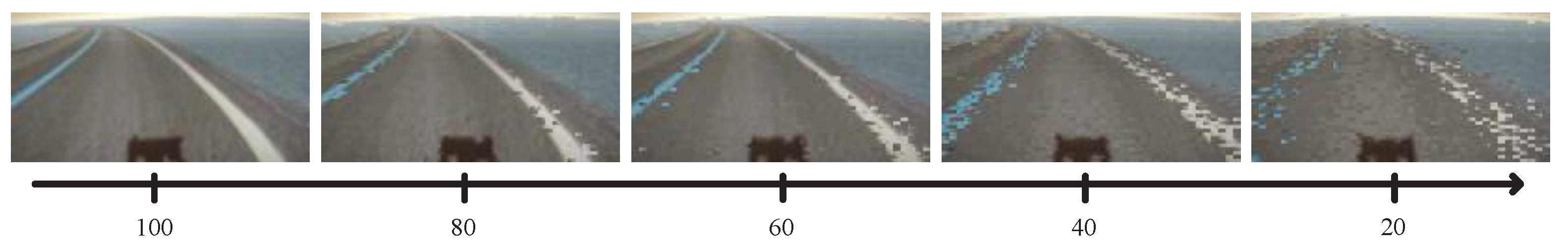
- We show the competitive performance of the D2WIN framework compared to baseline algorithms under various experiment settings. We also apply the framework in a car driving simulator, and demonstrate that the driving agent yields stable performance (i.e., 96.2% in the driving score) under highly limited resource conditions such as 70% suppression of sensor updates (i.e., only 30% resource usage; Section 4).
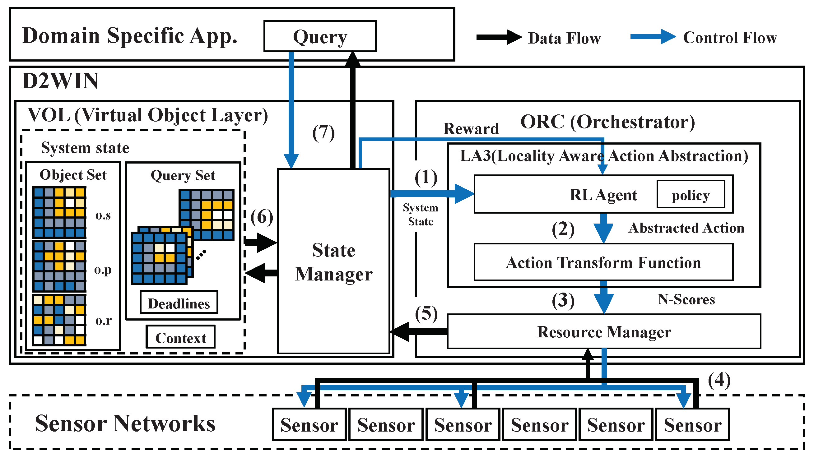
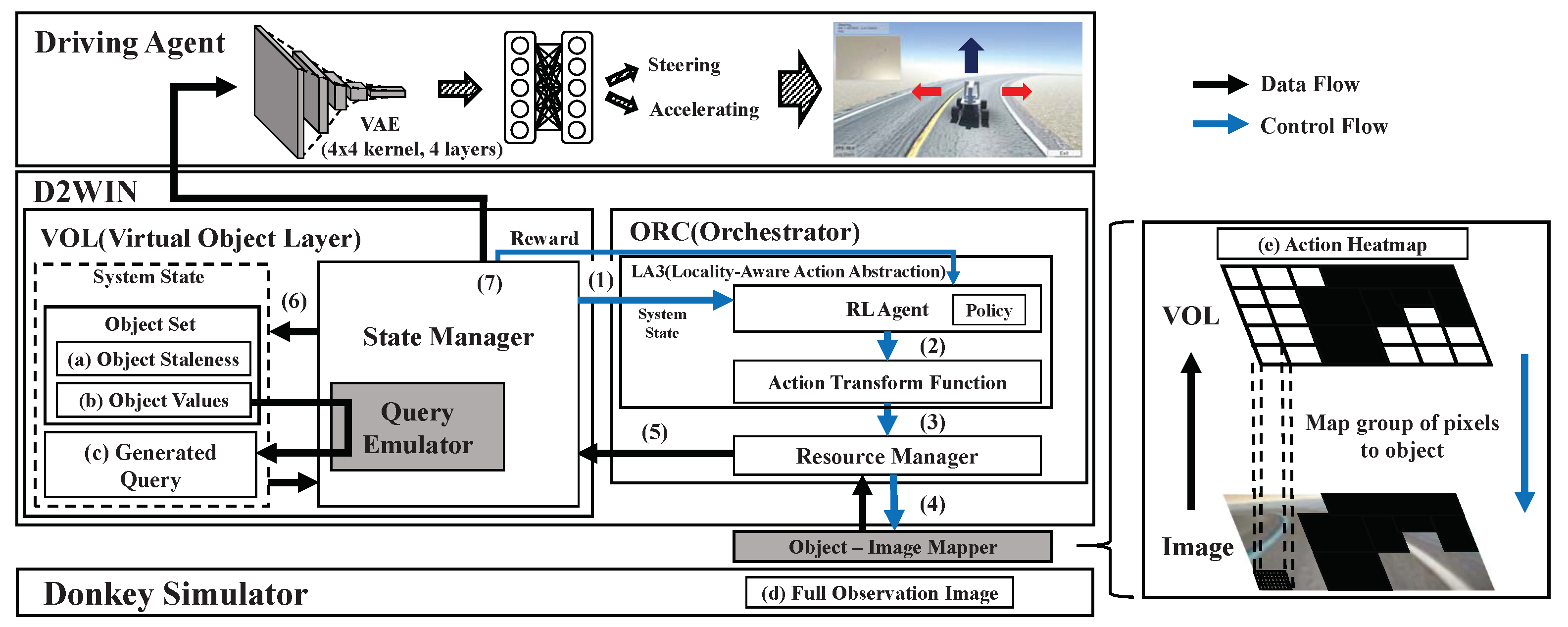
2. Framework Architecture
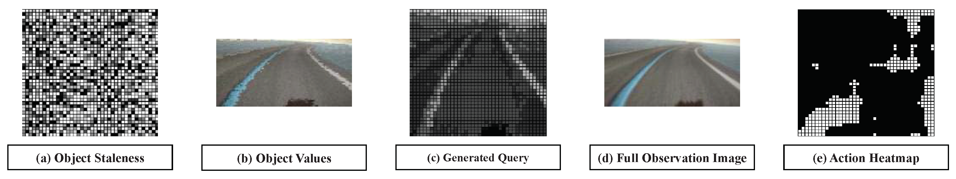
2.1. Virtual Object Layer for Sensor Data Management
2.2. RL-Based Data Orchestrator
| Algorithm 1: State manager process | |
| 1 | // initialize the system state |
| 2whiledo | |
| 3 | // (1)–(5) in Figure 4 |
| 4 for do | // (6) in Figure 4 |
| 5 | |
| 6 for do | |
| 7 , | // apply the result of job w |
| 8 | |
| 9 | |
| 10 for do | |
| 11 | |
| 12 for do | |
| 13 if then | |
| 14 ; | |
| 15 if then | |
| 16 , | |
| 17 else | |
| 18 | |
| 19 if then | |
| 20 , | |
| 21 | |
| 22 | // (7) in Figure 4 |
| 23 | |
3. Scheduling with Scalable Action Embedding
3.1. Scalable Action Embedding for Sensor Data Management
- is continuous on . Based on this definition, for small , there exists whenever implies , with the given metric on the virtual object space . That is, nearby objects o and rank closely because the function reflects the locality of sensor data.
- If we consider set C, the collection of local maximal points of , and the dimension of virtual object space d (note that we assume d = 2 for simplicity), then we have of measure zero [21] in the action space in , where is the Lebesgue measure in . It should be noted that object-wise selection by ranking is generally confined within the neighborhoods of the local maxima, and this property renders objects likely to be distinct in term of their ranking around the local maxima.
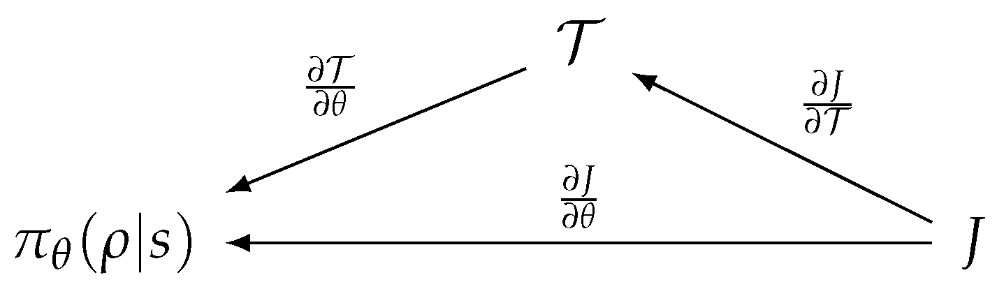
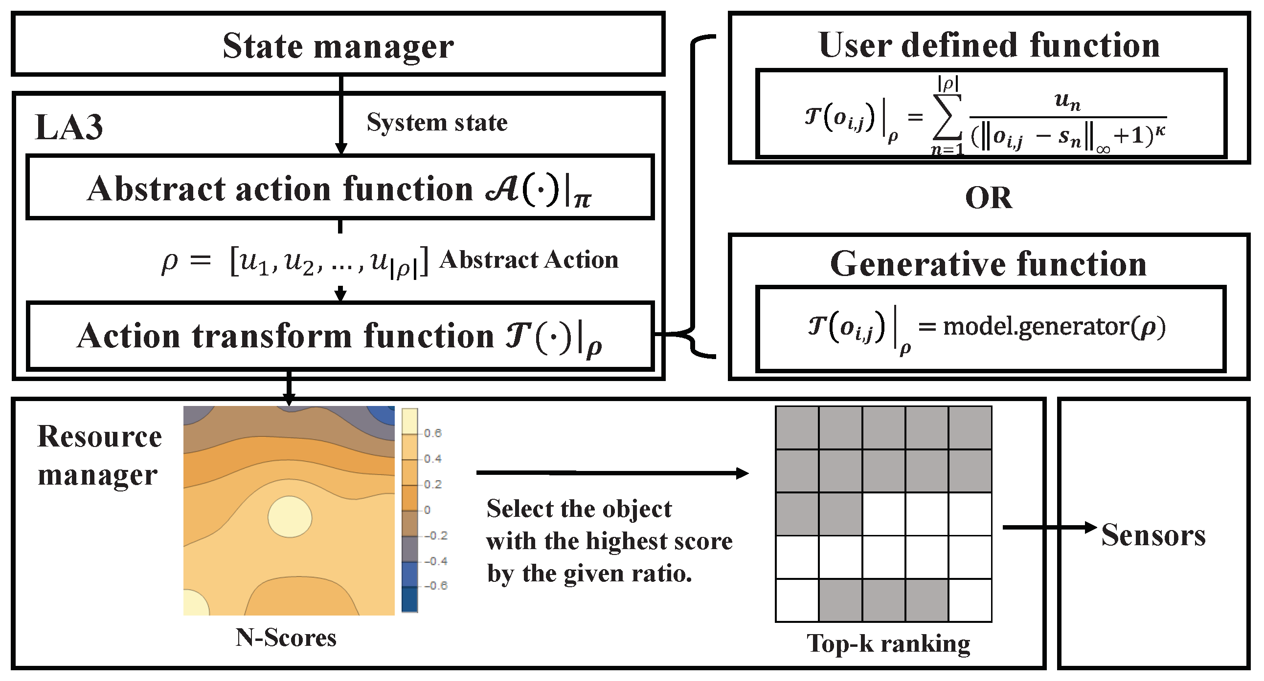
- The derivative of must be bounded. This condition is required to keep the RL score function differentiable and for its derivative to be confined within a stable range. RL algorithms then work as if no transformation of actions are involved in learning. Figure 6 depicts the procedure used to compute the derivative of the score function J of the RL algorithm. is a policy of the RL algorithm equipped with the weight , where s denotes the system state and denotes the abstract action. is a rewritten form of the action transform function, , obtained by currying.
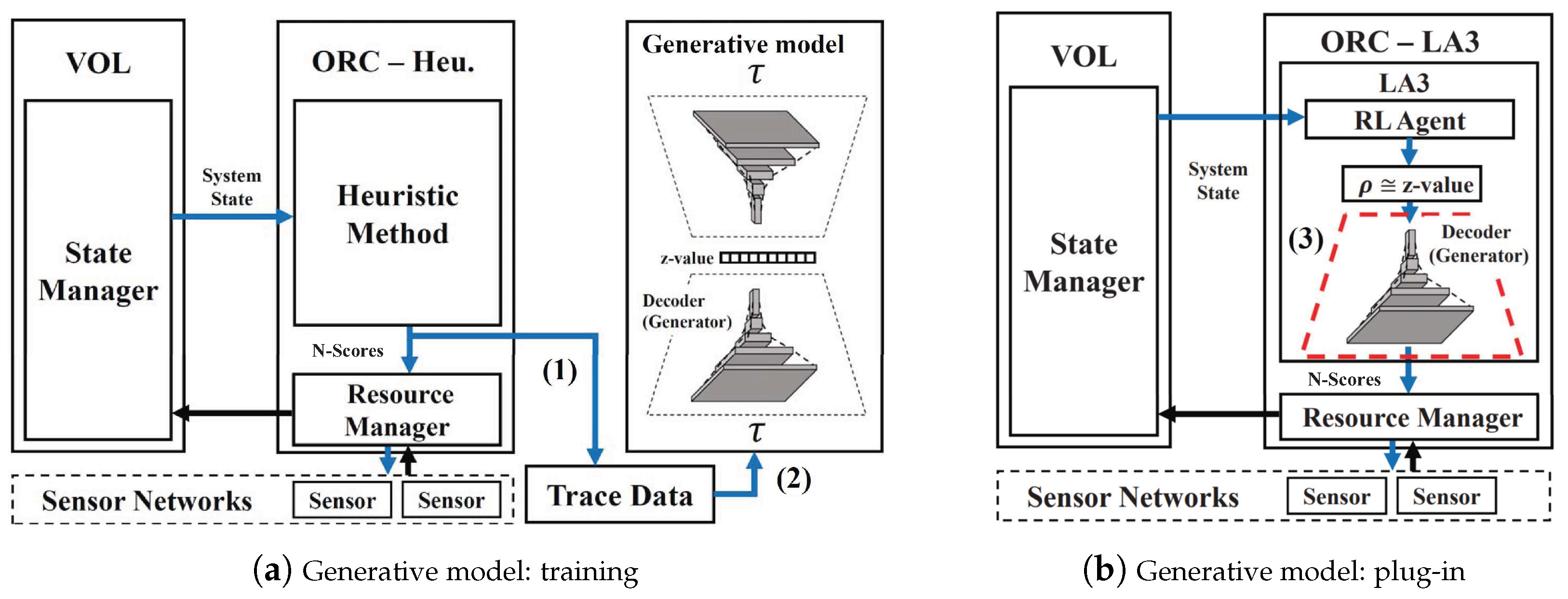
3.2. Learning-Based Action Transformation
| Algorithm 2:LA3 generalization process | |
| 1() | |
| 2 | // (1) use ORC’s heuristic method, e.g., SOF |
| 3←∅ | |
| 4whiledo | |
| 5 - | |
| 6 | |
| 7 .step(N-) | |
| 8.fit() | // (2) train the generative model |
| 9 | // (3) |
4. Evaluation
4.1. RL Implementation
4.2. Environment Implementation
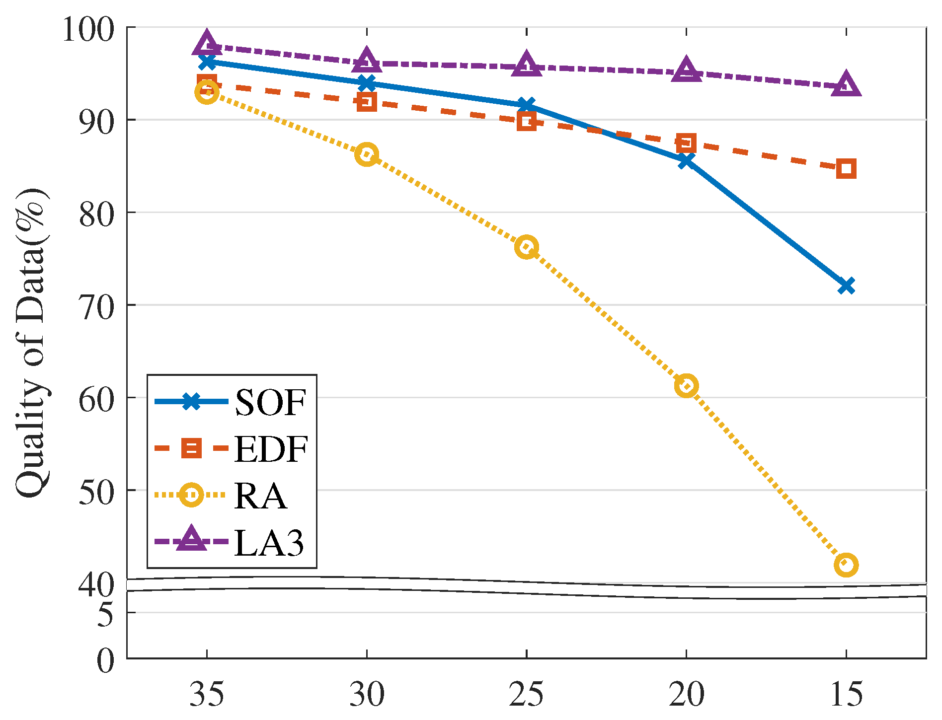
4.3. Model Evaluation
4.4. Case Study
4.4.1. Test System Implementation
4.4.2. Test System Evaluation
5. Related Work
6. Conclusions
Author Contributions
Funding
Conflicts of Interest
References
- Bradley, J.; Atkins, E. Optimization and Control of Cyberphysical Vehicle Systems. Sensors 2015, 15, 23020–23049. [Google Scholar] [CrossRef] [PubMed]
- Uhlemann, T.; Lehmann, C.; Steinhilper, R. The Digital Twin: Realizing the Cyber-Physical Production System for Industry 4.0. Procedia CIRP 2017, 61, 335–340. [Google Scholar] [CrossRef]
- Madni, A.M.; Madni, C.C.; Lucero, S.D. Leveraging Digital Twin Technology in Model-Based Systems Engineering. Systems 2019, 7, 7. [Google Scholar] [CrossRef]
- Uhlemann, T.; Schock, C.; Lehmann, C.; Freiberger, S.; Steinhilper, R. The Digital Twin: Demonstrating the Potential of Real Time Data Acquisition in Production Systems. Procedia Manuf. 2017, 9, 113–120. [Google Scholar] [CrossRef]
- Deshpande, A.; Guestrin, C.; Madden, S.R.; Hellerstein, J.M.; Hong, W. Model-driven Data Acquisition in Sensor Networks. In Proceedings of the Thirtieth International Conference on Very Large Data Bases, Toronto, ON, Canada, 31 August–3 September 2004. [Google Scholar]
- Donkey Simulator. Available online: https://docs.donkeycar.com/guide/simulator/ (accessed on 30 July 2019).
- Deshpande, A.; Madden, S. MauveDB: supporting model-based user views in database systems. In Proceedings of the 2006 ACM SIGMOD International Conference on Management of Data, Chicago, IL, USA, 27–29 June 2006; pp. 73–84. [Google Scholar]
- Morison, A.M.; Murphy, T.; Woods, D.D. Seeing Through Multiple Sensors into Distant Scenes: The Essential Power of Viewpoint Control. In Proceedings of the International Conference Human-Computer Interaction Platforms and Techniques, Toronto, ON, Canada, 17–22 July 2016; pp. 388–399. [Google Scholar]
- Autopilot. Available online: https://www.tesla.com/autopilot?redirect=no (accessed on 17 August 2019).
- Airsim Image APIs. Available online: https://microsoft.github.io/AirSim/docs/image_apis/ (accessed on 18 August 2019).
- Peng, Z.; Cui, D.; Zuo, J.; Li, Q.; Xu, B.; Lin, W. Random task scheduling scheme based on reinforcement learning in cloud computing. Cluster Comput. 2015, 18, 1595–1607. [Google Scholar] [CrossRef]
- Bao, Y.; Peng, Y.; Wu, C. Deep Learning-based Job Placement in Distributed Machine Learning Clusters. In Proceedings of the IEEE Conference on Computer Communications, Paris, France, 29 April–2 May 2019; pp. 505–513. [Google Scholar]
- Mao, H.; Alizadeh, M.; Menache, I.; Kandula, S. Resource management with deep reinforcement learning. In Proceedings of the 15th ACM Workshop on Hot Topics in Networks, Atlanta, GA, USA, 9–10 November 2016; pp. 50–56. [Google Scholar]
- Mao, H.; Schwarzkopf, M.; Venkatakrishnan, S.B.; Meng, Z.; Alizadeh, M. Learning Scheduling Algorithms for Data Processing Clusters. In Proceedings of the ACM Special Interest Group on Data Communication (SIGCOMM), Beijing, China, 19–24 August 2019; pp. 270–288. [Google Scholar]
- Chinchali, S.; Hu, P.; Chu, T.; Sharma, M.; Bansal, M.; Misra, R.; Pavone, M.; Katti, S. Cellular Network Traffic Scheduling with Deep Reinforcement Learning. In Proceedings of the Thirty-Second AAAI Conference on Artificial Intelligence, New Orleans, LA, USA, 2–7 February 2018. [Google Scholar]
- Krishnan, S.; Yang, Z.; Goldberg, K.; Hellerstein, J.M.; Stoica, I. Learning to Optimize Join Queries with Deep Reinforcement Learning. arXiv 2018, arXiv:1808.03196. [Google Scholar]
- Kang, K.D.; Son, S.H.; Stankovic, J.A. Managing deadline miss ratio and sensor data freshness in real-time databases. IEEE Trans. Knowl. Data Eng. 2004, 16, 1200–1216. [Google Scholar] [CrossRef]
- Zhou, Y.; Kang, K.D. Deadline assignment and tardiness control for real-time data services. In Proceedings of the 2010 22nd Euromicro Conference on Real-Time Systems, Brussels, Belgium, 6–9 July 2010; pp. 100–109. [Google Scholar]
- Sutton, R.S.; Barto, A.G. Reinforcement Learning: An Introduction; MIT Press: London, UK, 1998. [Google Scholar]
- Dulac-Arnold, G.; Evans, R.; van Hasselt, H.; Sunehag, P.; Lillicrap, T.; Hunt, J.; Mann, T.; Weber, T.; Degris, T.; Coppin, B. Deep reinforcement learning in large discrete action spaces. arXiv 2015, arXiv:1512.07679. [Google Scholar]
- Bartle, R.G.; Bartle, R.G. The Elements of Integration and Lebesgue Measure; A Wiley-Interscience: New York, NY, USA, 1995. [Google Scholar]
- Ho, J.; Ermon, S. Generative adversarial imitation learning. In Advances in Neural Information Processing Systems; Neural Information Processing Systems Foundation: Barcelona, Spain, 2016; pp. 4565–4573. [Google Scholar]
- TensorFlow. Available online: https://www.tensorflow.org (accessed on 30 July 2019).
- Haarnoja, T.; Zhou, A.; Abbeel, P.; Levine, S. Soft Actor-Critic: Off-Policy Maximum Entropy Deep Reinforcement Learning with a Stochastic Actor. arXiv 2018, arXiv:1801.01290. [Google Scholar]
- Schulman, J.; Wolski, F.; Dhariwal, P.; Radford, A.; Klimov, O. Proximal Policy Optimization Algorithms. arXiv 2017, arXiv:1707.06347. [Google Scholar]
- Duan, Y.; Chen, X.; Houthooft, R.; Schulman, J.; Abbeel, P. Benchmarking deep reinforcement learning for continuous control. In Proceedings of the 33rd International International Conference on Machine Learning (ICML), New York, NY, USA, 19–24 June 2016; pp. 1329–1338. [Google Scholar]
- Ramamritham, K. Real-time databases. Distrib. Parallel Databases 1993, 1, 199–226. [Google Scholar] [CrossRef]
- Zhou, Y.; Kang, K. Deadline Assignment and Feedback Control for Differentiated Real-Time Data Services. IEEE Trans. Knowl. Data Eng. 2015, 27, 3245–3257. [Google Scholar] [CrossRef]
- Mnih, V.; Heess, N.; Graves, A.; Kavukcuoglu, K. Recurrent models of visual attention. In Proceedings of the Advances in Neural Information Processing Systems, Montreal, QC, Canada, 8–13 December 2014; pp. 2204–2212. [Google Scholar]
- Elgabli, A.; Khan, H.; Krouka, M.; Bennis, M. Reinforcement Learning Based Scheduling Algorithm for Optimizing Age of Information in Ultra Reliable Low Latency Networks. arXiv 2018, arXiv:1811.06776. [Google Scholar]
- Chowdhury, A.; Raut, S.A.; Narman, H.S. DA-DRLS: Drift adaptive deep reinforcement learning based scheduling for IoT resource management. J. Netw. Comput. Appl. 2019, 138, 51–65. [Google Scholar] [CrossRef]
- Pazis, J.; Parr, R. Generalized value functions for large action sets. In Proceedings of the 28th International Conference on Machine Learning (ICML-11), Bellevue, WA, USA, 28 June–2 July 2011; pp. 1185–1192. [Google Scholar]
- Sallab, A.E.; Abdou, M.; Perot, E.; Yogamani, S. Deep reinforcement learning framework for autonomous driving. Electron. Imaging 2017, 2017, 70–76. [Google Scholar] [CrossRef]
- Using Keras and Deep Deterministic Policy Gradient to Play TORCS. Available online: https://yanpanlau.github.io/2016/10/11/Torcs-Keras.html (accessed on 30 July 2019).
- Mnih, V.; Badia, A.P.; Mirza, M.; Graves, A.; Lillicrap, T.; Harley, T.; Silver, D.; Kavukcuoglu, K. Asynchronous methods for deep reinforcement learning. In Proceedings of the 33rd International Conference on Machine Learning (ICML), New York, NY, USA, 19–24 June 2016; pp. 1928–1937. [Google Scholar]
- Li, D.; Zhao, D.; Zhang, Q.; Chen, Y. Reinforcement Learning and Deep Learning Based Lateral Control for Autonomous Driving [Application Notes]. IEEE Comput. Intell. Mag. 2019, 14, 83–98. [Google Scholar] [CrossRef]
- Kaushik, M.; Prasad, V.; Krishna, K.M.; Ravindran, B. Overtaking maneuvers in simulated highway driving using deep reinforcement learning. In Proceedings of the 2018 IEEE Intelligent Vehicles Symposium (IV), Changshu, China, 26–30 June 2018; pp. 1885–1890. [Google Scholar]
- Wu, K.; Abolfazli Esfahani, M.; Yuan, S.; Wang, H. Learn to steer through deep reinforcement learning. Sensors 2018, 18, 3650. [Google Scholar] [CrossRef] [PubMed]
- Zhou, X.; Gao, Y.; Guan, L. Towards goal-directed navigation through combining learning based global and local planners. Sensors 2019, 19, 176. [Google Scholar] [CrossRef] [PubMed]
- TORCS—The Open Racing Car Simulator. Available online: https://sourceforge.net/projects/torcs/ (accessed on 30 July 2019).
- Jaritz, M.; de Charette, R.; Toromanoff, M.; Perot, E.; Nashashibi, F. End-to-end race driving with deep reinforcement learning. In Proceedings of the 2018 IEEE International Conference on Robotics and Automation (ICRA), Brisbane, Australia, 21–26 May 2018; pp. 2070–2075. [Google Scholar]


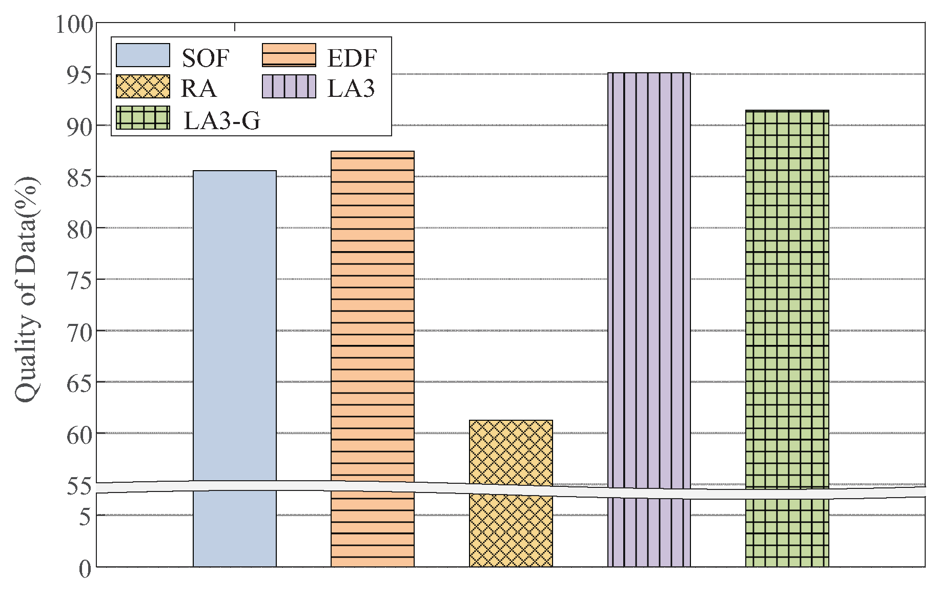
| Models | Description |
|---|---|
| Stalest Object First (SOF) | selection in the staleness order |
| Earliest Deadline First (EDF) | selection in the deadline order |
| Random Action (RA) | selection by random fixed point values |
| Locality-Aware Action Abstraction (LA3) | selection by RL agent with action transform function |
| Hyperparameter | Description : Training RL (SAC and PPO) | Value | |
|---|---|---|---|
| SAC | PPO | ||
| State | Object set, Query set, Context | ||
| Action | Parameter (Abstract action) | ||
| Reward evaluation | Satisfied query : +, Violated query : – | ||
| Network layer structure | MLP(2 Layer, [64, 64]) with layer normalisation | ||
| Action transform function | The function converts an abstract action into ranking | User defined function (Equation (2)) | |
| Discount factor () | The constant for reflect future reward | 0.99 | |
| Learning rate () | The learning rate | 0.0001 | 0.00025 |
| Training frequency | The number of timesteps between updating the model | 1 | - |
| Gradient steps | The number of gradient descent steps in update | 1 | - |
| Batch size | The size of batch. In PPO, batch size is as follows: (number of agents) × (number of steps per update) | 64 | 8 * 128 |
| Replay buffer size | The size of replay buffer | 50,000 | - |
| Target smoothing coef. | The soft update coefficient | 0.005 | - |
| GAE parameter | The Generalized Advantage Estimator | - | 0.95 |
| VF coef. | The value function coefficient for loss calculation | - | 0.5 |
| Clipping estimator | The clipping range parameter | - | 0.2 |
| Hyperparameter | Description : Training generative model (VAE) | Value | |
| Network layer structure | VAE (3 convolution layers; filter size: 3 × 3; stride: 1; number of filters: [64, 32, 16]) | ||
| Learning rate () | The learning rate | 0.00025 | |
| Optimizer | The method of updating NN | Adam | |
| Latent dimension | The dimension of the output of the encoder in VAE | 12 | |
| Sample size | The number of data in the data set | 50,000 | |
| Epoch | The number of learning for the entire data set in NN | 20 | |
| Description | Value (Default) | |
|---|---|---|
| VOL scale | The number of virtual objects | , , , , , , () |
| managed by VOL | ||
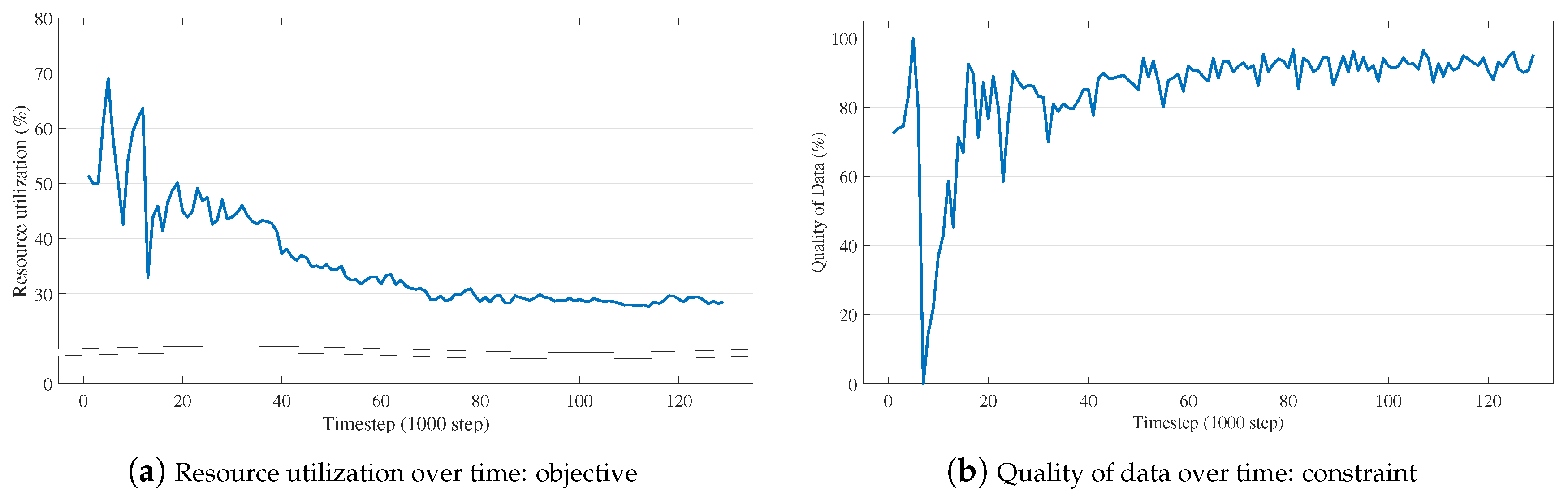
| Resource limit | Rate of usable resources (%) | 35, 30, 25, 20, 15 (20) |
| Query arrival rate | The average of query arrival in | 1, 2, 3, 4, 5 (1) |
| a Poisson distribution () | ||
| Query dynamics | The expected spatial difference | 30, 45, 60, 75 (45) |
| between two consecutive queries (%) |
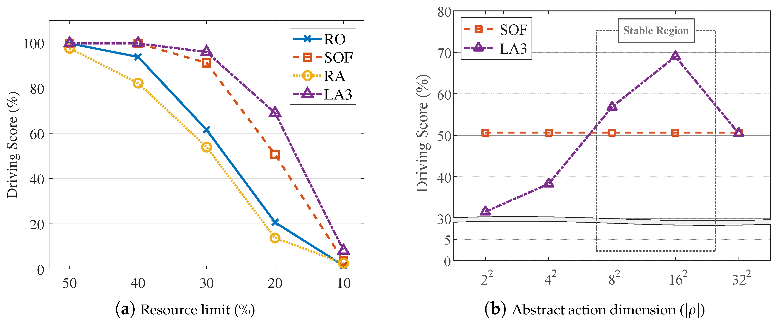
| Description | Value (Default) | |
|---|---|---|
| Resource limit | Rate of usable resources (%) | 50, 40, 30, 20, 10 (20) |
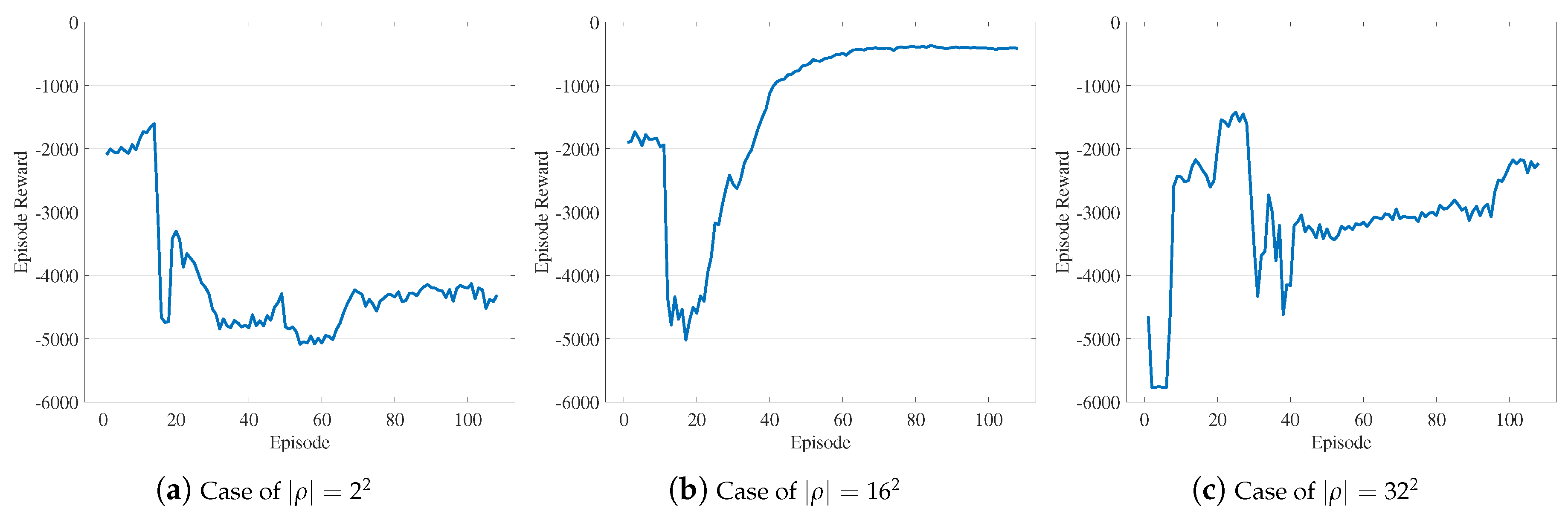
| The size of | The dimension of abstract actions | , , , , () |
© 2019 by the authors. Licensee MDPI, Basel, Switzerland. This article is an open access article distributed under the terms and conditions of the Creative Commons Attribution (CC BY) license (http://creativecommons.org/licenses/by/4.0/).
Share and Cite
Jeong, S.; Yoo, G.; Yoo, M.; Yeom, I.; Woo, H. Resource-Efficient Sensor Data Management for Autonomous Systems Using Deep Reinforcement Learning. Sensors 2019, 19, 4410. https://doi.org/10.3390/s19204410
Jeong S, Yoo G, Yoo M, Yeom I, Woo H. Resource-Efficient Sensor Data Management for Autonomous Systems Using Deep Reinforcement Learning. Sensors. 2019; 19(20):4410. https://doi.org/10.3390/s19204410
Chicago/Turabian StyleJeong, Seunghwan, Gwangpyo Yoo, Minjong Yoo, Ikjun Yeom, and Honguk Woo. 2019. "Resource-Efficient Sensor Data Management for Autonomous Systems Using Deep Reinforcement Learning" Sensors 19, no. 20: 4410. https://doi.org/10.3390/s19204410
APA StyleJeong, S., Yoo, G., Yoo, M., Yeom, I., & Woo, H. (2019). Resource-Efficient Sensor Data Management for Autonomous Systems Using Deep Reinforcement Learning. Sensors, 19(20), 4410. https://doi.org/10.3390/s19204410