A Transductive Model-based Stress Recognition Method Using Peripheral Physiological Signals

Abstract
1. Introduction
- (1)
- For the first process, few recent efforts have measured the relevant data in high dimensions, but rather they have depended on the clustering before training. This means that the correlation measurement is performed in the low-dimensional space, whilst the linear prediction is performed in the high-dimensional space, which may cause the hyperplane to be affected by unfiltered outliers. Regarding the support vector regression (SVR), the outliers, meaning the irrelevant data, may lead to serious consequences [23].
- (2)
- For the second process, these studies rely on the widely used inductive reasoning, based on global optimization, and they only consider processing the training set instead of the test instances. Inductive reasoning is based on learning from experience, which aims to generate meanings from the training set to identify patterns and relationships to build a recognition model. It is useful for a global model of the approximate problem, but for each individual case, it does not have good generalization ability.
- (1)
- We proposed a transductive model to reduce the generalization error for stress recognition from the peripheral physiological signals;
- (2)
- Extracting the non-linear peripheral physiological features, which can characterize the time-frequency features of small sliding windows to better support real-time stress recognition;
- (3)
- The performance of the proposed method was investigated on the self-established database, as well as the widely used DEAP dataset [27]. The results indicated that our method outperformed the existing methods.
- (4)
- The real interactive experiment was performed to explore the feasibility of this framework based on non-invasive sensors.
2. Related Work
2.1. Sensor-based Physiological Signals
2.2. Transductive Learning
2.3. Stress Recognition
3. Data Collection and Assessment Methodology
3.1. Participants
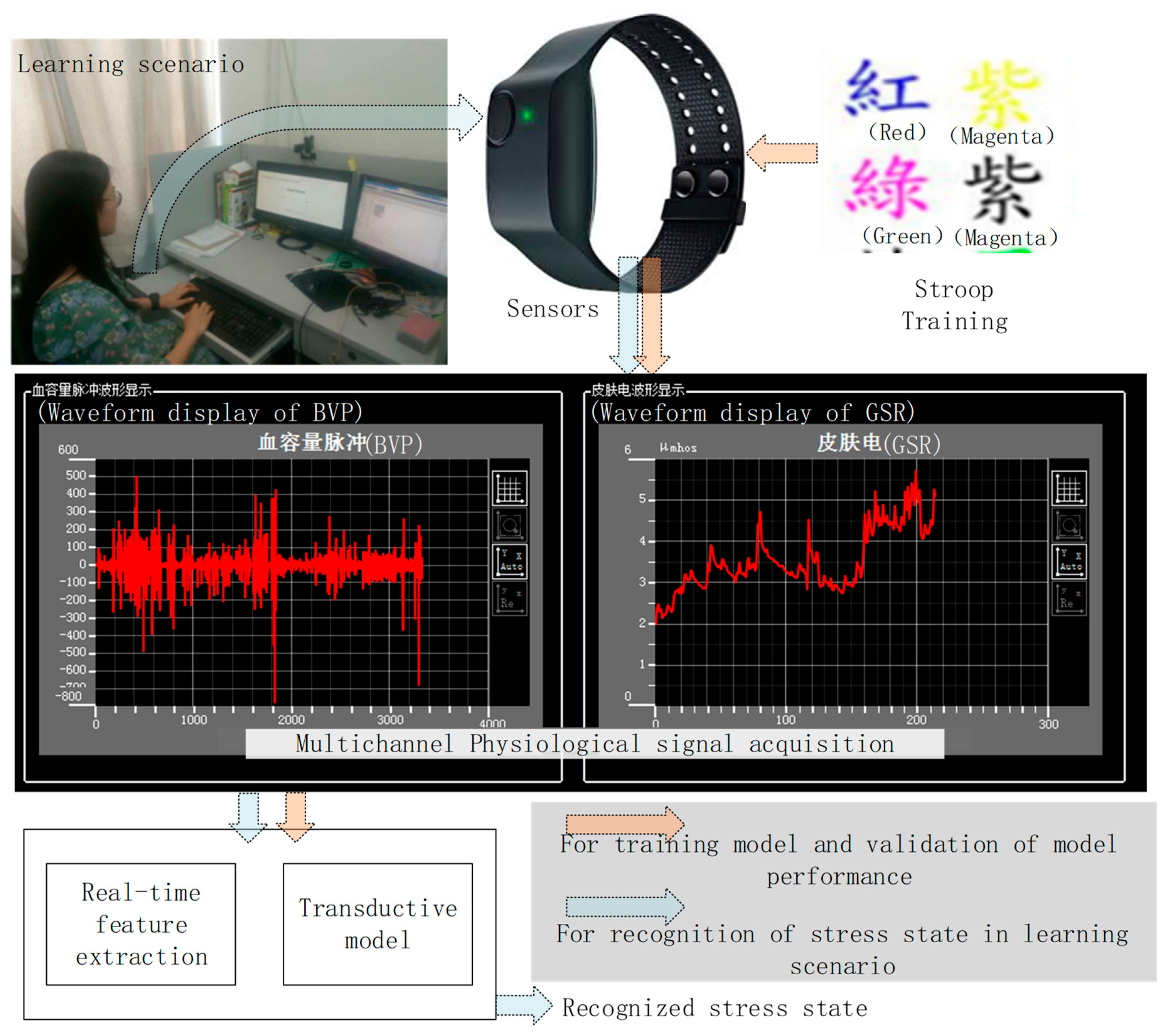
3.2. Stroop Training
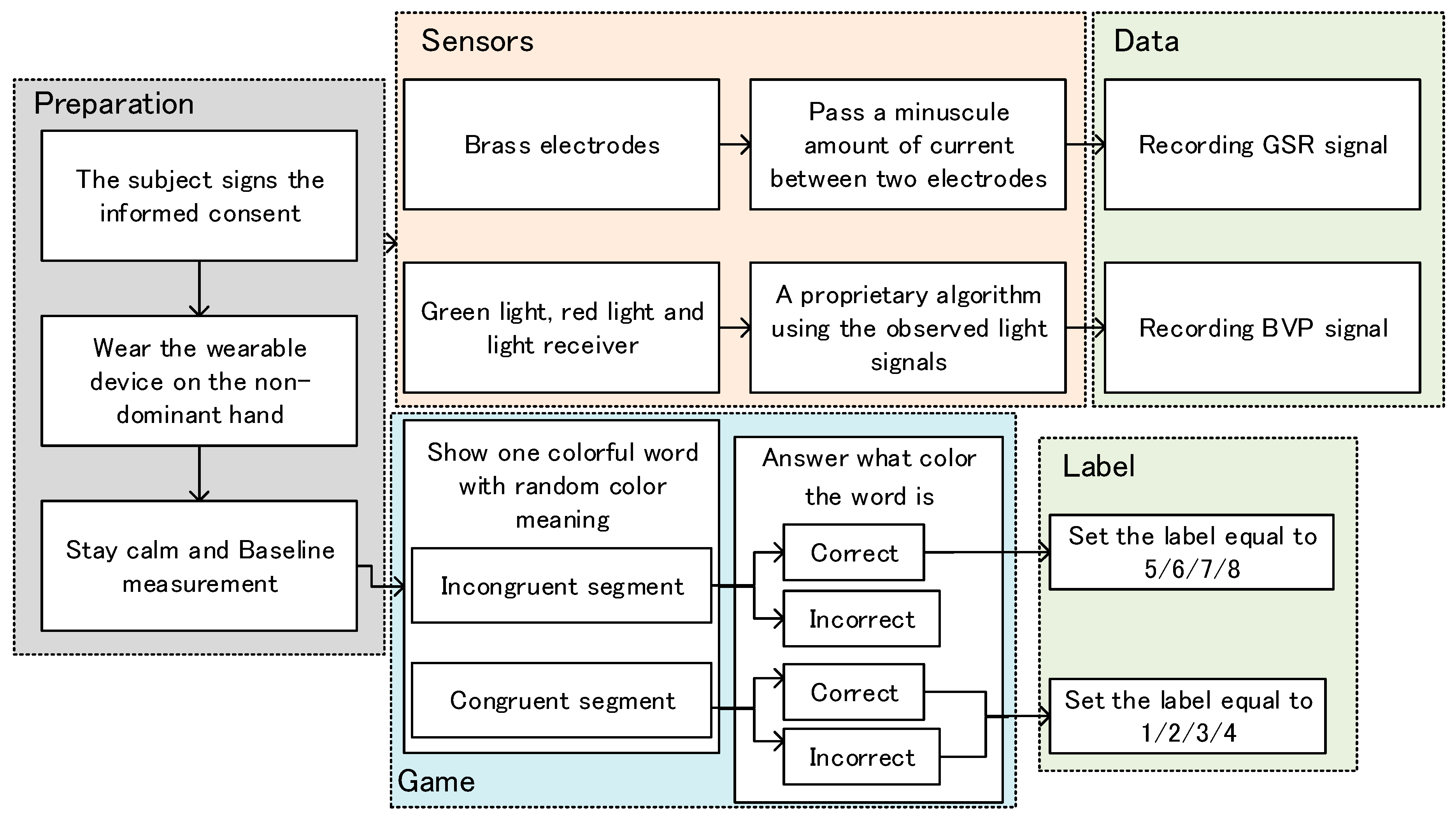
- (1)
- The subjects signed the consent forms.
- (2)
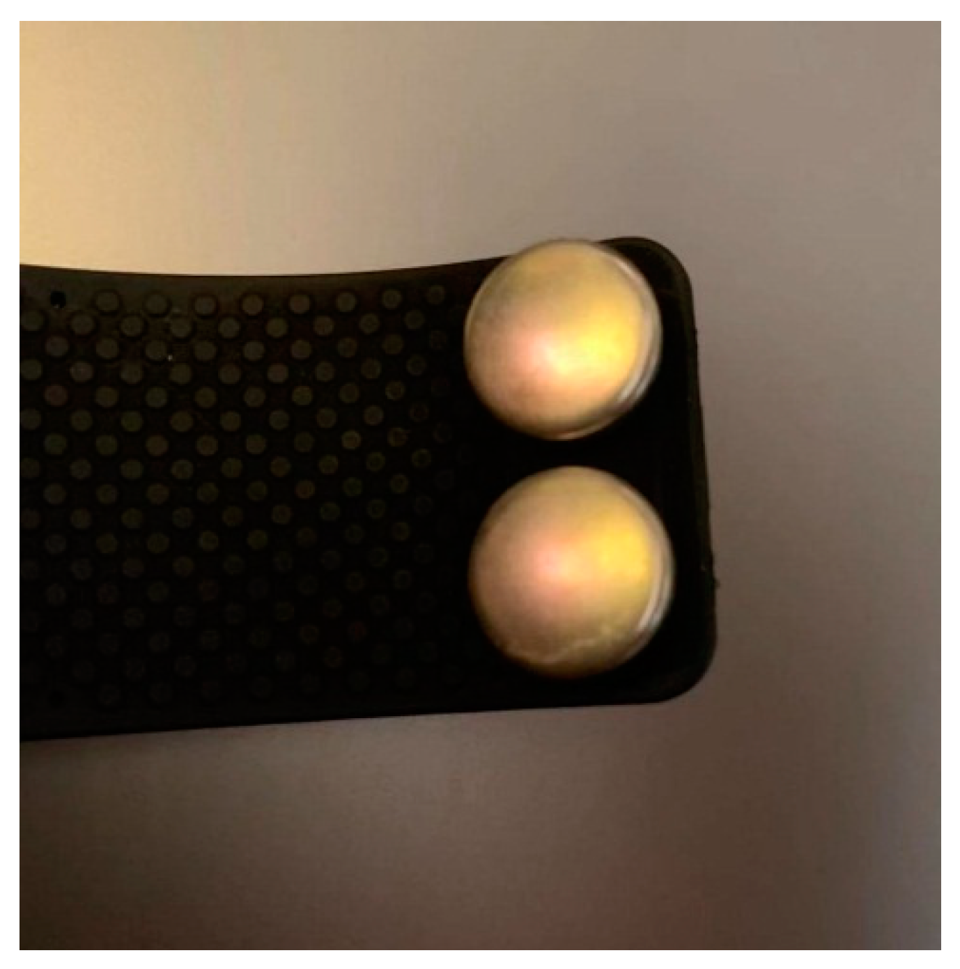
- The subjects wore the wearable device on the non-dominant wrist, for recording the GSR and BVP signals simultaneously. The technical documentation [43] from Emaptica was strictly followed for recording the signals effectively.
- (3)
- The subjects were asked to stay calm for a period of the baseline measurement.
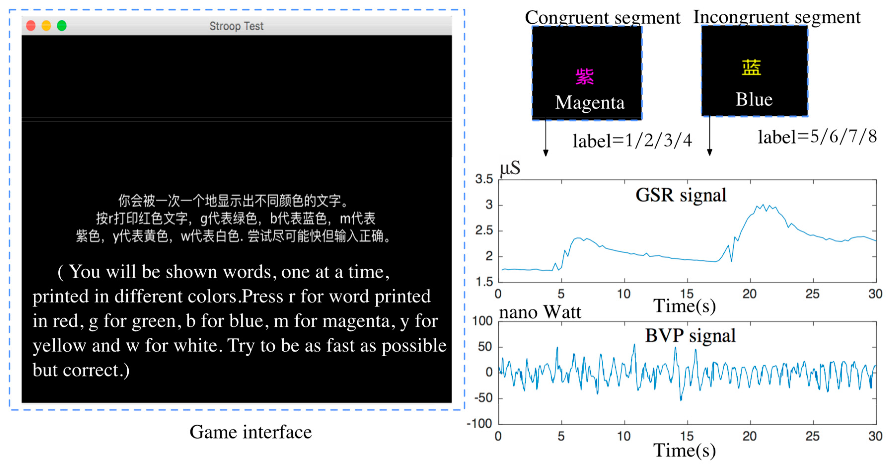
- (4)
- After the game started, the PC screen displayed a word, the meaning of which was one kind of color, and its font color was random.
- (5)
- Subjects were asked to select the correct key that represented the font color instead of the word meaning. They would wait 2 seconds and then the next word was taken.
- (6)
- The difficulty of the game ranged from simple to difficult, with four levels. Each level has 40 words. The game at the simple level waited longer for the answers, and vice versa.
- (7)
- When the answer time was exceeded, the next word was taken, and the previous word was treated as an incorrect answer.
3.3. Learning Scenario
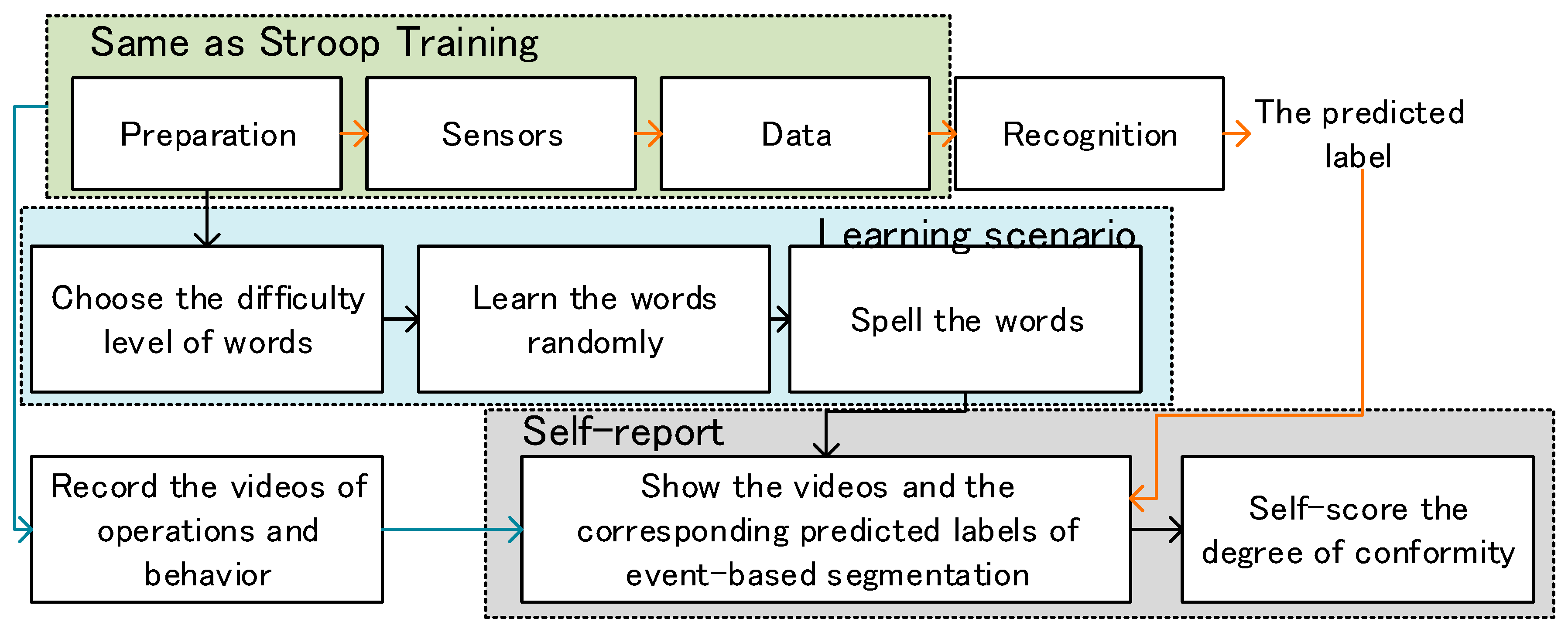
- (1)
- The processes of preparation, sensors and data acquisition were the same as Stroop training.
- (2)
- There are three processes involved in learning scenario as shown in Figure 5. The order of words set randomly in advance was the same for each subject in each process.
- (3)
- The words without meaning were shown successively and the subjects selected the difficulty level of each word quickly.
- (4)
- The subjects learned each word with meaning within one minute. And each subject need to learn 60 words.
- (5)
- The interactive interface only showed the meaning of each word and the subjects were required to spell the words within a limited time. The interactive interface is shown in Appendix B.
4. The Stress Recognition Methodology
4.1. Peripheral Physiological Features
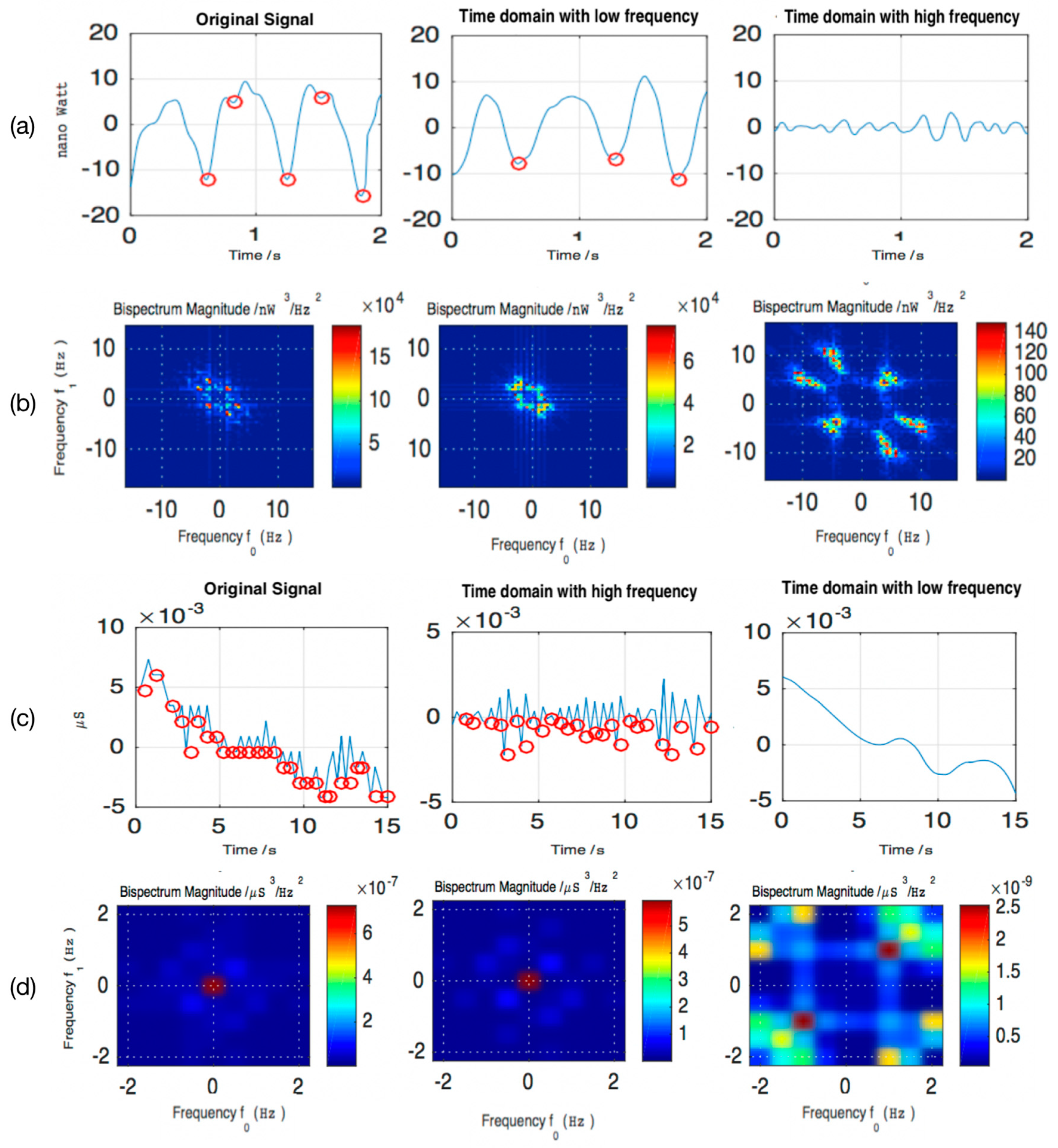
4.1.1. BVP Signals
4.1.2. GSR Signals
4.1.3. Extracted Features
4.2. Transductive Model
5. Results
5.1. Transdutive model
5.1.1. Overview
Benchmark
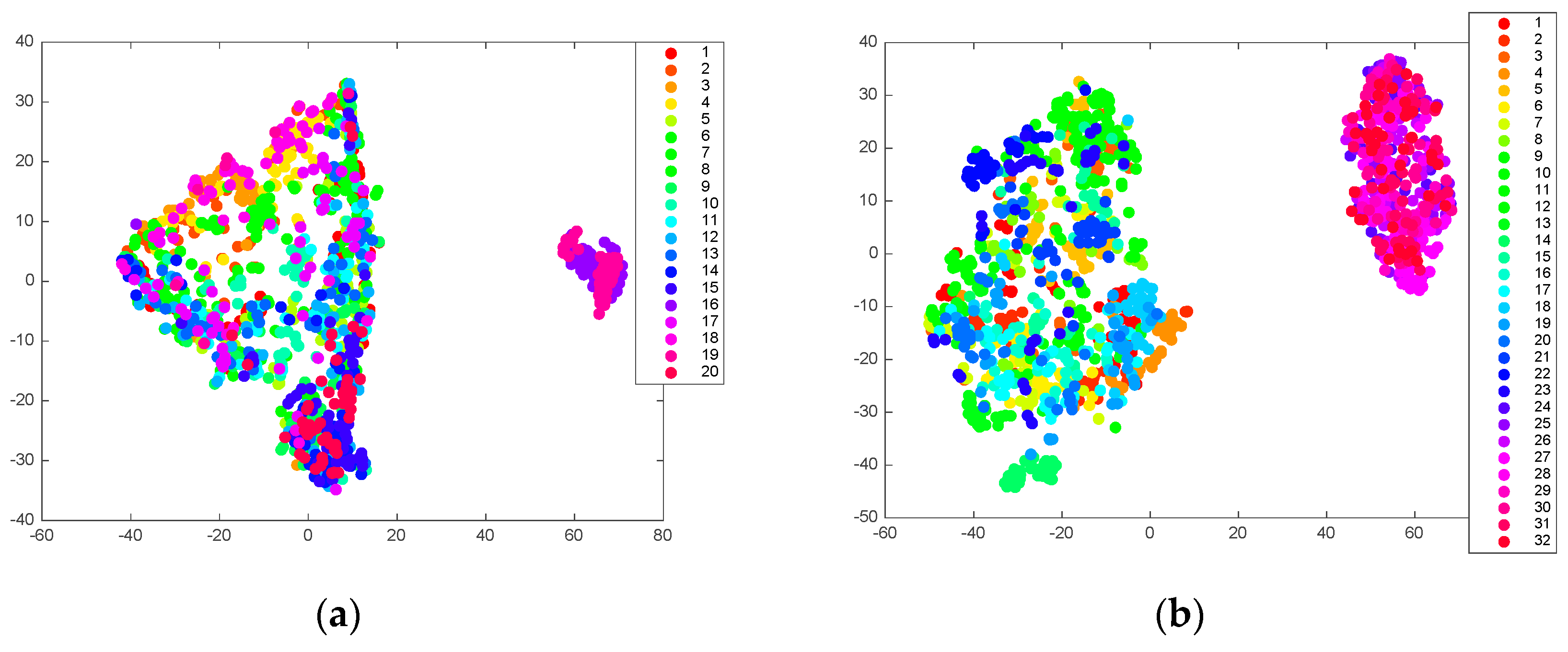
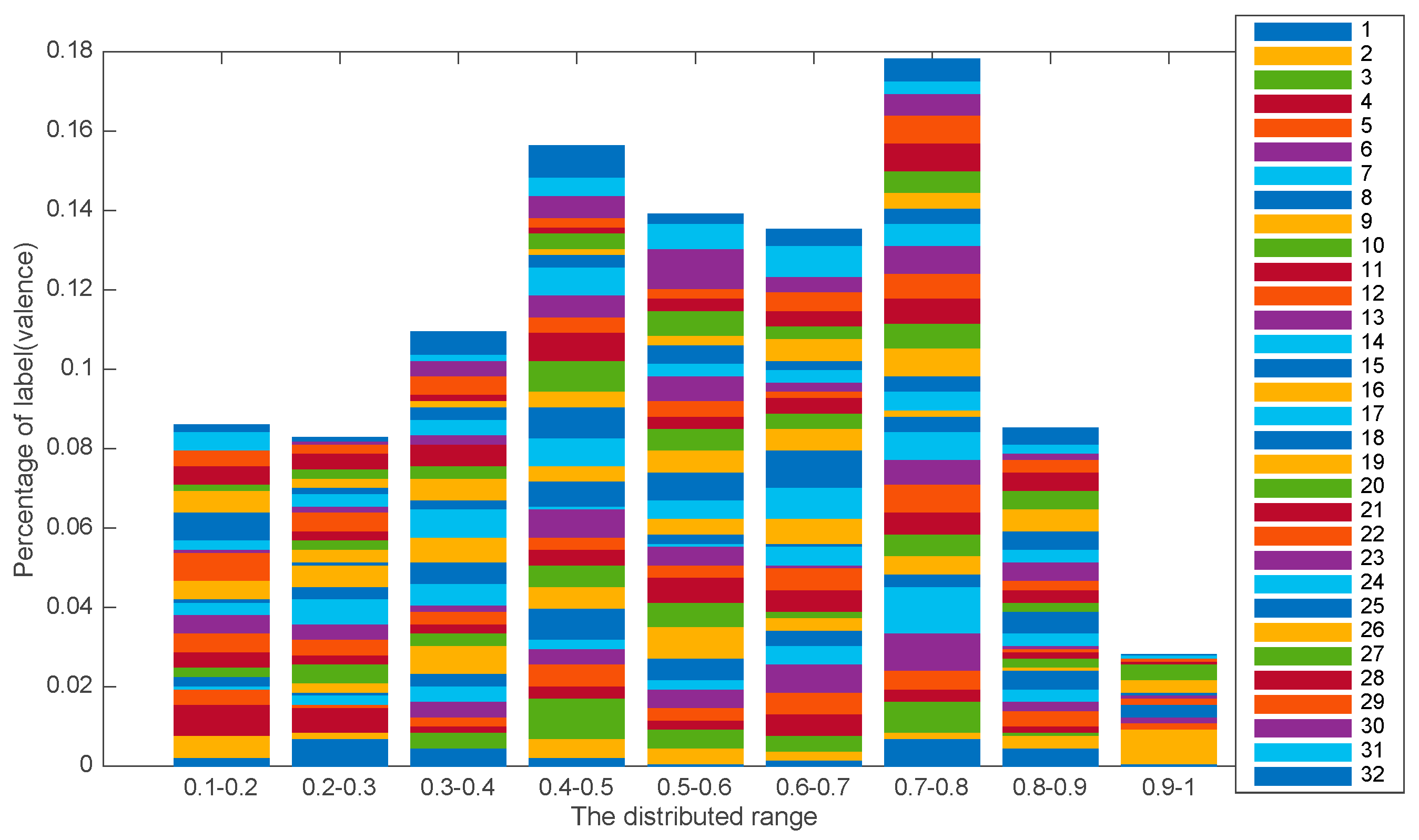
Data Distribution
Compared models
- e-SVR and LR: Due to the dispersed data distribution, training the data from all subjects could not reach the state of convergence. Therefore, the data from one subject was used to train one model.
- CNN: We used an individual subject for training the CNN using the original GSR and BVP input. Like the EEG signal for prediction using CNN [56], the GSR and BVP could be treated as two channels from the EEG for independent CNN training, and then the two outputs were concatenated to input the fully connected layer. Moreover, the output layer’s activation function was a linear function, as in Reference [57].
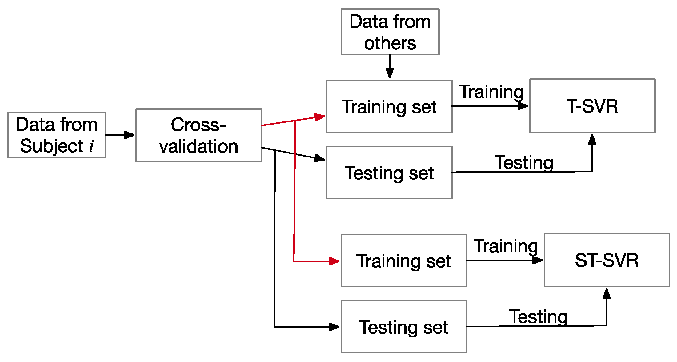
- ST-SVR: This differentiates the categories for training. As shown in Figure 8, the ST-SVR uses each subject’s individual examples to train the models. The training set and the test set of the subject i is divided by the cross-validation from subject i’s dataset.
- T-SVR: Involves training without distinction. For subject i, the T-SVR uses all the subjects’ examples to train the model, except the testing set from subject i.
Hyperparameters
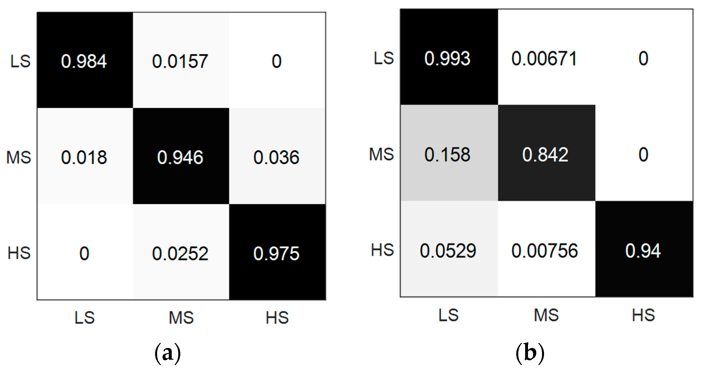
5.1.2. Stroop Training Results
5.1.3. DEAP Dataset Results
5.1.4. Comparison of Stroop Training and DEAP Dataset Results
5.1.5. Comparison to State-of-the-Art Results
5.2. Learning Scenario
- (1)
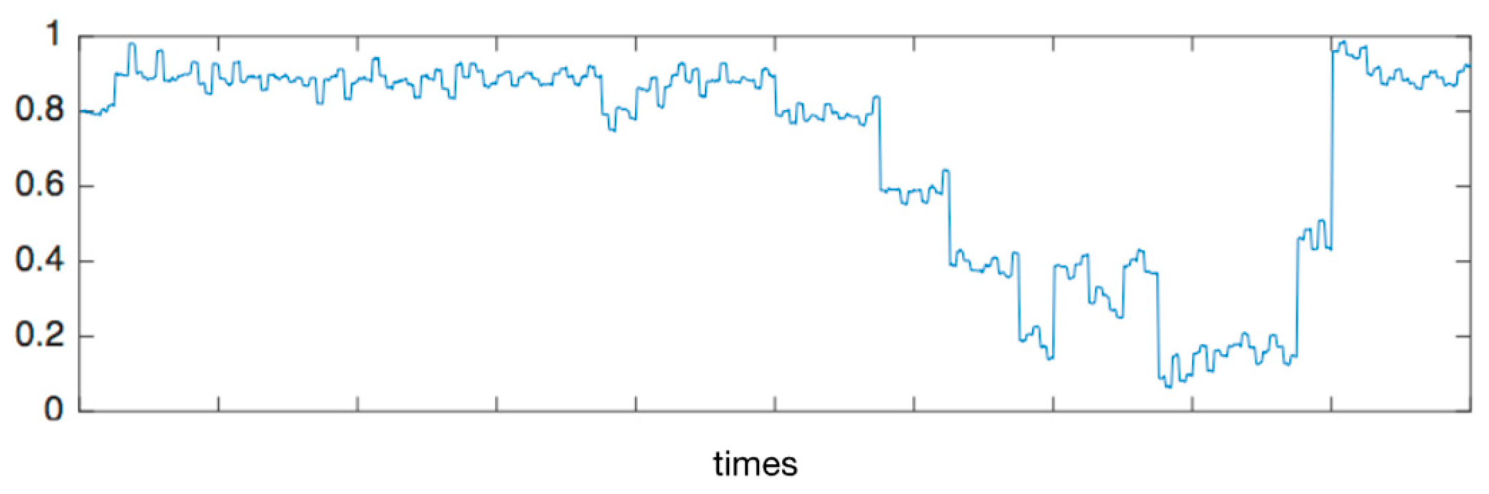
- Both the difficult and easy questions had a similar mean and similar SD of the CD. It indicated the reliability of the real-time stress recognition.
- (2)
- The ratio of the number of high stress to the number of low stress was 1.79 during the difficult questions period, whilst the ratio was 0.52 during the easy questions period. It could be concluded that the difficult questions led to more stress.
6. Discussion
- We provided a transductive model, considering about the clustering methods based on neighborhood knowledge in high dimension.
- A field study was presented in learning scenario, using non-linear features, based on non-invasive wearable device.
6.1. Discussion of Transductive Model
- (1)
- Few studies of stress recognition provided the description of the data distribution, which had a great influence on the recognition performance.
- (2)
- The annotation method is different, including the self-report or automatic labelling.
- (3)
- The difference in the underlying sensors causes the reliability of the received physiological signals to be unevaluable.
- (1)
- The lower accuracy of the concurrent label than the self-assessment may be an important reason.
- (2)
- Stroop training has a larger label granularity than the DEAP. Intuitively, the identified labels could also have larger intervals.
- (3)
- The sliding window size was different. DEAP has a 1-minute signal length which may more fully characterize the psycho–physiological regular pattern.
6.2. Discussion of Learning scenario
7. Conclusions
Author Contributions
Funding
Conflicts of Interest
Appendix A

Appendix B

References
- Rani, P.; Sarkar, N.; Adams, J. Anxiety-based affective communication for implicit human-machine interaction. Adv. Eng. Inform. 2007, 21, 323–334. [Google Scholar] [CrossRef]
- Sun, F.T.; Kuo, C.; Cheng, H.T.; Buthpitiya, S.; Collins, P.; Griss, M. Activity-aware mental stress detection using physiological sensors. In Proceedings of the 2nd International Conference on Mobile Computing, Applications and Services, Santa Clara, CA, USA, 25–28 October 2010; pp. 282–301. [Google Scholar]
- Xu, Q.; Tin, L.W.; Guan, C. Cluster-based analysis for personalized stress evaluation using physiological signals. IEEE J. Biomed. Health Inform. 2015, 19, 275–281. [Google Scholar] [CrossRef] [PubMed]
- Daglarli, E.; Temeltas, H.; Yesiloglu, M. Behavioral task processing for cognitive robots using artificial emotions. Neurocomputing 2009, 72, 2835–2844. [Google Scholar] [CrossRef]
- Gerald, O.; James, J.G. The Senses Considered as Perceptual Systems. Leonardo 1966, 1, 89. [Google Scholar]
- Belkaid, M.; Cuperlier, N.; Gaussier, P. Emotional modulation of peripersonal space as a way to represent reachable and comfort areas. In Proceedings of the IEEE/RSJ International Conference on Intelligent Robots and Systems, Hamburg, Germany, 28 September–2 October 2015; pp. 353–359. [Google Scholar]
- Ben-Zeev, D.; Scherer, E.A.; Wang, R.; Xie, H.; Campbell, A.T. Next-generation psychiatric assessment: Using smartphone sensors to monitor behavior and mental health. Psychiatr. Rehabil. J. 2015, 38, 218. [Google Scholar] [CrossRef] [PubMed]
- Shu, L.; Xie, J.; Yang, M.; Yang, M.; Li, Z.; Li, Z.; Liao, D.; Xu, X.; Yang, X. A review of emotion recognition using physiological signals. Sensors 2018, 18, 2074. [Google Scholar] [CrossRef] [PubMed]
- Singh, M.; Yadav, K.; Kumar, A.; Madhu, H.J.; Mukherjee, T. Method and device for non-invasive monitoring of physiological parameters. U.S. Patent US20170105681A1, 20 April 2017. [Google Scholar]
- Parlak, O.; Keene, S.T.; Marais, A.; Curto, V.F.; Salleo, A. Molecularly selective nanoporous membrane-based wearable organic electrochemical device for noninvasive cortisol sensing. Sci. Adv. 2018, 4, eaar2904. [Google Scholar] [CrossRef] [PubMed]
- Bandodkar, A.J.; Jeerapan, I.; Wang, J. Wearable chemical sensors: Present challenges and future prospects. ACS Sens. 2016, 1, 464–482. [Google Scholar] [CrossRef]
- Bloss, R. Wearable sensors bring new benefits to continuous medical monitoring, real time physical activity assessment, baby monitoring and industrial applications. Sens. Rev. 2015, 35, 141–145. [Google Scholar] [CrossRef]
- Trung, T.Q.; Lee, N.-E. Flexible and stretchable physical sensor integrated platforms for wearable human-activity monitoring and personal healthcare. Adv. Mater. 2016, 28, 4338–4372. [Google Scholar] [CrossRef]
- Harris, W.S.; Schoenfeld, C.D.; Weissler, A.M. Effects of adrenergic receptor activation and blockade on the systolic preejection period, heart rate, and arterial pressure in man. Clin. Investig. 1967, 46, 1704–1714. [Google Scholar] [CrossRef] [PubMed]
- Reisman, S. Measurement of physiological stress. In Proceedings of the IEEE 23rd Northeast Bioengineering Conference, Durham, NH, USA, 21–22 May 1997; pp. 21–23. [Google Scholar]
- Liao, W.; Zhang, W.; Zhu, Z.; Ji, Q. A real-time human stress monitoring system using dynamic Bayesian network. In Proceedings of the IEEE Computer Society Conference on Computer Vision and Pattern Recognition (CVPR’05)—Workshops, San Diego, CA, USA, 21–23 September 2005. [Google Scholar]
- Garbarino, M.; Lai, M.; Bender, D.; Picard, R.W.; Tognetti, S. Empatica E3—A wearable wireless multi-sensor device for real-time computerized biofeedback and data acquisition. In Proceedings of the 2014 EAI 4th International Conference on Wireless Mobile Communication and Healthcare (Mobihealth), Athens, Greece, 3–5 November 2014; pp. 39–42. [Google Scholar]
- Fairclough, S.H. Fundamentals of physiological computing. Interact. Comput. 2009, 21, 133–145. [Google Scholar] [CrossRef]
- Hasegawa, Y.; Ootsuka, T.; Fukuda, T.; Arai, F.; Kawaguchi, M. A relaxation system adapting to user’s condition-identification of relationship between massage intensity and heart rate variability. In Proceedings of the IEEE International Conference on Robotics, Seoul, Korea, 21–26 May 2001; pp. 3195–3200. [Google Scholar]
- Zhang, B.; Morère, Y.; Sieler, L.; Langlet, C.; Bolmont, B.; Bourhis, G. Reaction time and physiological signals for stress recognition. Biomed. Signal Process. Control 2017, 38, 100–107. [Google Scholar] [CrossRef]
- Varvara, K.; Tayebi, N. A Controlled Set-Up Experiment to Establish Personalized Baselines for Real-Life Emotion Recognition. arXiv, 2017; arXiv:1703.06537. [Google Scholar]
- Khadidja, G.; Reguig, F.B.; Maaoui, C. Discrete wavelet transform analysis and empirical mode decomposition of physiological signals for stress recognition. Int. J. Biomed. Eng. Technol. 2018, 27, 247–270. [Google Scholar]
- Debruyne, M. An outlier map for support vector machine classification. Ann. Appl. Stat. 2009, 3, 1566–1580. [Google Scholar] [CrossRef]
- Vapnik, V. The Nature of Statistical Learning Theory, 2nd ed.; Springer: Berlin, Germany, 1999. [Google Scholar]
- Pang, S.; Ban, T.; Kadobayashi, Y.; Kasabov, N. Personalized mode transductive spanning SVM classification tree. Inf. Sci. 2011, 181, 2071–2085. [Google Scholar] [CrossRef]
- Gunnar, L.; Czyzykow-Czarnocka, S. Priming of the Emotional Stroop Effect by a Schema Questionnaire: An Experimental Study of Test Order. Cogn. Ther. Res. 2001, 25, 281–289. [Google Scholar]
- Koelstra, S.; Muhl, C.; Soleymani, M.; Lee, J.S.; Yazdani, A.; Ebrahimi, T.; Pun, T.; Nijholt, A.; Patras, I. DEAP: A Database for Emotion Analysis Using Physiological Signals. IEEE Trans. Affect. Comput. 2012, 3, 18–31. [Google Scholar] [CrossRef]
- Rahim, S.; Patel, C.; Kim, I. Non-contact Wearable EEG Sensors for SSVEP-based Brain Computer Interface Applications. In Proceedings of the 40th Annual International Conference of the IEEE Engineering in Medicine and Biology Society (EMBC), Honolulu, HI, USA, 17–21 July 2018; pp. 2016–2019. [Google Scholar]
- Yapici, M.K.; Tamador, E.A. Intelligent medical garments with graphene-functionalized smart-cloth ECG sensors. Sensors 2017, 17, 875. [Google Scholar] [CrossRef]
- Ammar, A.; Weber, W.M.; McHale, R.T. System and method for monitoring the life of a physiological sensor. U.S. Patent US7880626, 1 February 2011. [Google Scholar]
- Cheng, H.; Tan, P.N.; Jin, R. Efficient algorithm for localized support vector machine. IEEE Trans. Knowl. Data Eng. 2010, 22, 537–549. [Google Scholar] [CrossRef]
- Hakan, C.; Franc, V. Large-scale robust transductive support vector machines. Neurocomputing 2017, 235, 199–209. [Google Scholar]
- Li, Y.; Wang, Y.; Bi, C.; Jiang, X. Revisiting transductive support vector machines with margin distribution embedding. Knowl.-Based Syst. 2018, 152, 200–214. [Google Scholar] [CrossRef]
- Zimmermann, P.; Guttormsen, S.; Danuser, B.; Gomez, P. Affective Computing a Rationale for Measuring Mood With Mouse and Keyboard. Int. J. Occup. Saf. Ergon. 2003, 9, 539–551. [Google Scholar] [CrossRef] [PubMed]
- Hwang, B.; You, J.; Vaessen, T.; Myin-Germeys, I.; Park, C.; Zhang, B.T. Deep ECGNet: An Optimal Deep Learning Framework for Monitoring Mental Stress Using Ultra Short-Term ECG Signals. Telemed. J. E-Health 2018, 24, 753–772. [Google Scholar] [CrossRef] [PubMed]
- Cho, Y.; Bianchi-Berthouze, N.; Julier, S.J. DeepBreath: Deep learning of breathing patterns for automatic stress recognition using low-cost thermal imaging in unconstrained settings. In Proceedings of the 2017 Seventh International Conference on Affective Computing and Intelligent Interaction (ACII), Antonio, TX, USA, 23–26 October 2017; pp. 456–463. [Google Scholar]
- Lim, W.L.; Liu, Y.; Subramaniam, S.C.H.; Liew, S.H.P.; Krishnan, G.; Sourina, O.; Konovessis, D.; Ang, H.E.; Wang, L. EEG-Based Mental Workload and Stress Monitoring of Crew Members in Maritime Virtual Simulator. In Transactions on Computational Science XXXII; Gavrilova, M.L., Tan, C.J.K., Sourin, A., Eds.; Springer: Berlin, Germany, 2018; Volume 10830, pp. 15–28. ISBN 9783662566725. [Google Scholar]
- Giannakakis, G.; Pediaditis, M.; Manousos, D.; Kazantzaki, E.; Chiarugi, F.; Simos, P.G.; Marias, K.; Tsiknakis, M. Stress and anxiety detection using facial cues from videos. Biomed. Signal Process. Control 2017, 31, 89–101. [Google Scholar] [CrossRef]
- Mozos, O.M.; Sandulescu, V.; Andrews, S.; Ellis, D.; Bellotto, N.; Dobrescu, R.; Ferrandez, J.M. Stress detection using wearable physiological and sociometric sensors. Int. J. Neural Syst. 2017, 27, 1650041. [Google Scholar] [CrossRef] [PubMed]
- Ciabattoni, L.; Ferracuti, F.; Longhi, S.; Pepa, L.; Romeo, L.; Verdini, F. Real-time mental stress detection based on smartwatch. In Proceedings of the IEEE International Conference on Consumer Electronics (ICCE), Las Vegas, NV, USA, 8–11 January 2017; pp. 110–111. [Google Scholar]
- de Santos Sierra, A.; Ávila, C.S.; Casanova, J.G.; del Pozo, G.B. A stress-detection system based on physiological signals and fuzzy logic. IEEE Trans. Ind. Electron. 2011, 58, 4857–4865. [Google Scholar] [CrossRef]
- Zhai, J.; Barreto, A. Stress detection in computer users based on digital signal processing of noninvasive physiological variables. In Proceedings of the 28th International Conference of the IEEE Engineering in Medicine & Biology Society, New York, NY, USA, 31 August–3 September 2006; pp. 1355–1358. [Google Scholar]
- Wear Your E4 Wristband. Available online: https://support.empatica.com/hc/en-us/articles/206374015-Wear-your-E4-wristband- (accessed on 11 October 2018).
- Kivikangas, J.M.; Chanel, G.; Cowley, B.; Ekman, I.; Salminen, M.; Järvelä, S.; Ravaja, N. A review of the use of psychophysiological methods in game research. J. Gaming Virtual Worlds 2011, 3, 181–199. [Google Scholar] [CrossRef]
- Wu, S.; Lin, T. Exploring the use of physiology in adaptive game design. In Proceedings of the 2011 International Conference on Consumer Electronics, Communications and Networks (CECNet), Xianning, China, 11–13 March 2011; pp. 1280–1283. [Google Scholar]
- Mahmoud, M.; Baltrušaitis, T.; Robinson, P.; Riek, L.D. 3D corpus of spontaneous complex mental states. In Proceedings of the 4th International Conference on Affective Computing and Intelligent Interaction (ACII), Memphis, TN, USA, 9–12 October 2011; pp. 205–214. [Google Scholar]
- He, L.; Jiang, D.; Yang, L.; Pei, E.; Wu, P.; Sahli, H. Multimodal affective dimension prediction using deep bidirectional long short-term memory recurrent neural networks. In Proceedings of the 5th International Workshop on Audio/Visual Emotion Challenge, Brisbane, Australia, 26–30 October 2015; pp. 73–80. [Google Scholar]
- Van Aelst, S. Stahel–Donoho estimation for high-dimensional data. Int. J. Comput. Math. 2016, 93, 628–639. [Google Scholar] [CrossRef]
- Brown, C.C.; Raio, C.M.; Neta, M. Cortisol responses enhance negative valence perception for ambiguous facial expressions. Sci. Rep. 2017, 7, 15107. [Google Scholar] [CrossRef]
- Liapis, A.; Katsanos, C.; Sotiropoulos, D.G.; Karousos, N.; Xenos, M. Stress in interactive applications: Analysis of the valence-arousal space based on physiological signals and self-reported data. Multimedia Tools Appl. 2017, 76, 5051–5071. [Google Scholar] [CrossRef]
- Maaten, L.; Hinton, G. Visualizing data using t-SNE. J. Mach. Learn. Res. 2008, 9, 2579–2605. [Google Scholar]
- Germine, L.T.; Hooker, C.I. Face emotion recognition is related to individual differences in psychosis-proneness. Psychol. Med. 2011, 41, 937. [Google Scholar] [CrossRef] [PubMed]
- Chen, Y.A.; Wang, J.C.; Yang, Y.H.; Chen, H. Linear regression-based adaptation of music emotion recognition models for personalization. In Proceedings of the IEEE International Conference on Acoustics, Speech and Signal Processing, Florence, Italy, 4–9 May 2014; pp. 2149–2153. [Google Scholar]
- Saffer, H.; Dave, D.; Grossman, M.; Ann Leung, L. Racial, Ethnic, and Gender Differences in Physical Activity. J. Hum. Cap. 2013, 7, 378–410. [Google Scholar] [CrossRef] [PubMed]
- Chang, C.C.; Lin, C.J. LIBSVM: A library for support vector machines. ACM Trans. Intell. Syst. Technol. 2011, 2, 1–27. [Google Scholar] [CrossRef]
- Hajinoroozi, M.; Mao, Z.; Jung, T.P.; Lin, C.T.; Huang, Y. EEG-based prediction of driver’s cognitive performance by deep convolutional neural network. Signal Process. Image Commun. 2016, 47, 549–555. [Google Scholar] [CrossRef]
- Shimobaba, T.; Kakue, T.; Ito, T. Convolutional neural network-based regression for depth prediction in digital holography. arXiv, 2018; arXiv:1802.00664. [Google Scholar]
- Martinez, R.; Irigoyen, E.; Arruti, A.; Martín, J.I.; Muguerza, J. A real-time stress classification system based on arousal analysis of the nervous system by an F-state machine. Comput. Methods Prog. Biomed. 2017, 148, 81–90. [Google Scholar] [CrossRef] [PubMed]


| Cha. | Feature | Description |
|---|---|---|
| BVP | Diastolic point (Low frequency) | The mean and SD of IBI |
| Spectral features | The value of 1 in low frequency | |
| Statistical moments (Low frequency) | Mean and SD of signal | |
| GSR | Peaks (High/Low frequency) | The number and amplitude of peaks |
| Spectral features | The value of in low and high frequency | |
| Statistical moments (High/Low frequency) | Mean and SD of the first derivation, the second derivation, and negative slope [47] |
| -SVR | Linear Regression | CNN | ST-SVR | T-SVR | ||
|---|---|---|---|---|---|---|
| Absolute Error | MAE | 0.250 | 0.256 | 0.231 | 0.193 | 0.213 |
| SD | 0.091 | 0.101 | 0.082 | 0.061 | 0.069 | |
| Time (ms) | Mean | 3.69 | 0.40 | 322.90 | 63.34 | 121.67 |
| SD | 0.20 | 0.03 | 43.16 | 11.29 | 38.92 | |
| -SVR | Linear Regression | CNN | ST-SVR | T-SVR | ||
|---|---|---|---|---|---|---|
| Absolute Error | MAE | 0.183 | 0.198 | 0.181 | 0.156 | 0.162 |
| SD | 0.054 | 0.060 | 0.052 | 0.043 | 0.046 | |
| Time (ms) | Mean | 0.52 | 1.01 | 201.55 | 28.98 | 41.53 |
| SD | 0.17 | 0.67 | 50.14 | 9.34 | 13.67 | |
| QA-FSM | ST-SVR | T-SVR | |
|---|---|---|---|
| Training Mode | Subject-dependent | Subject-dependent | Subject-independent |
| LS | 0.943 | 0.987 | 0.929 |
| MS | 0.970 | 0.943 | 0.903 |
| HS | 0.984 | 0.975 | 0.969 |
| Standard of Question | Stress > 0.5 | Stress ≤ 0.5 | Correct | Incorrect | Answering Time(s) | CD | |
|---|---|---|---|---|---|---|---|
| Number | |||||||
| Difficult | 388 | 217 | 577 | 28 | Mean | 17.26 | 85% |
| SD | 22.44 | 13.8% | |||||
| Easy | 101 | 194 | 200 | 95 | Mean | 15.80 | 84.95% |
| SD | 17.45 | 13.3% | |||||
© 2019 by the authors. Licensee MDPI, Basel, Switzerland. This article is an open access article distributed under the terms and conditions of the Creative Commons Attribution (CC BY) license (http://creativecommons.org/licenses/by/4.0/).
Share and Cite
Li, M.; Xie, L.; Wang, Z. A Transductive Model-based Stress Recognition Method Using Peripheral Physiological Signals. Sensors 2019, 19, 429. https://doi.org/10.3390/s19020429
Li M, Xie L, Wang Z. A Transductive Model-based Stress Recognition Method Using Peripheral Physiological Signals. Sensors. 2019; 19(2):429. https://doi.org/10.3390/s19020429
Chicago/Turabian StyleLi, Minjia, Lun Xie, and Zhiliang Wang. 2019. "A Transductive Model-based Stress Recognition Method Using Peripheral Physiological Signals" Sensors 19, no. 2: 429. https://doi.org/10.3390/s19020429
APA StyleLi, M., Xie, L., & Wang, Z. (2019). A Transductive Model-based Stress Recognition Method Using Peripheral Physiological Signals. Sensors, 19(2), 429. https://doi.org/10.3390/s19020429