HEALPix-IA: A Global Registration Algorithm for Initial Alignment


Abstract
1. Introduction
2. Related Works
3. Problem Formulation
4. HEALPix-IA Algorithm
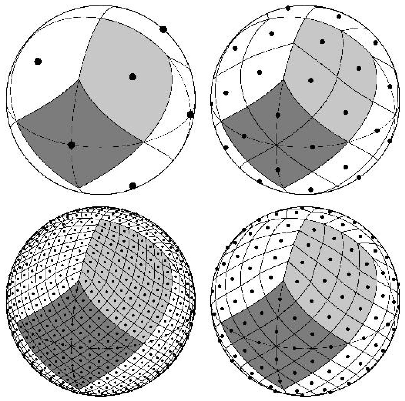
4.1. Pixelization, Projection and Indexing
4.2. Point Correspondence Searching
4.3. Point Correspondence Optimization
4.4. Rotation Estimation
| Algorithm 1: Estimate and optimize the corresponding points. | ||
| input: ModelS and DataT with normals of size (N is the scale of Model/Data) | ||
| output: 2 pairs of corresponding points , , and | ||
| 1 | extract normals and from S and T | |
| 2 | ; ; | // see Equations (7) & (8) |
| 3 | forto 12 do | |
| 4 | ; | // maximum intensity and the index |
| 5 | ||
| 6 | ; ; | // normals of the max |
| 7 | ; ; | // see Equation (6) |
| 8 | construct Struct | |
| 9 | end for | |
| 10 | sortrows (; ) sortrows (); | // descending sort |
| 11 | ||
| 12 | ||
| 13 | whiledo | // see Eqution (10) |
| 14 | ||
| 15 | ||
| 16 | end while | |
| 17 | ||
| 18 | forto 12 do | |
| 19 | ||
| 20 | if then | // see Equation (12) |
| 21 | ||
| 22 | break; | |
| 23 | end if | |
| 24 | end for | |
| 25 | let then calculate ; | // see Equation (13) |
| 26 | ||
| 27 | create in plane A then | |
| 28 | ; | // project normals to A |
| 29 | calculate ; | // see Equation (14) |
| 30 | mesh region into 100 grids; | |
| 31 | search with the peak intensity in meshed grids; | |
| 32 | calculate inverse projection point | |
| 33 | calculate , , | |
4.5. Correlation Searching
| Algorithm 2: Optimal transformation search. | ||
| input: ModelS and DataT with normals of size (N is the scale of Model/Data) | ||
| output: transformation T, correlation , iteration | ||
| 1 | initialize | |
| 2 | extract normals and from S and T | |
| 3 | ; | // see Equation (8) |
| 4 | while and do | |
| 5 | estimate initial transformation with Equations (15)∼(18) | |
| 6 | ||
| 7 | calculate ; | // see Equation (19) |
| 8 | ||
| 9 | if then | |
| 10 | if then | |
| 11 | ||
| 12 | end if | |
| 13 | ||
| 14 | ||
| 15 | ||
| 16 | end if | |
| 17 | if and then | |
| 18 | ; | // see Equation (20) |
| 19 | ||
| 20 | ||
| 21 | end if | |
| 22 | ||
| 23 | end while | |
5. Results and Evaluation
5.1. Simulation
5.1.1. Compared with EGI-Based Methods
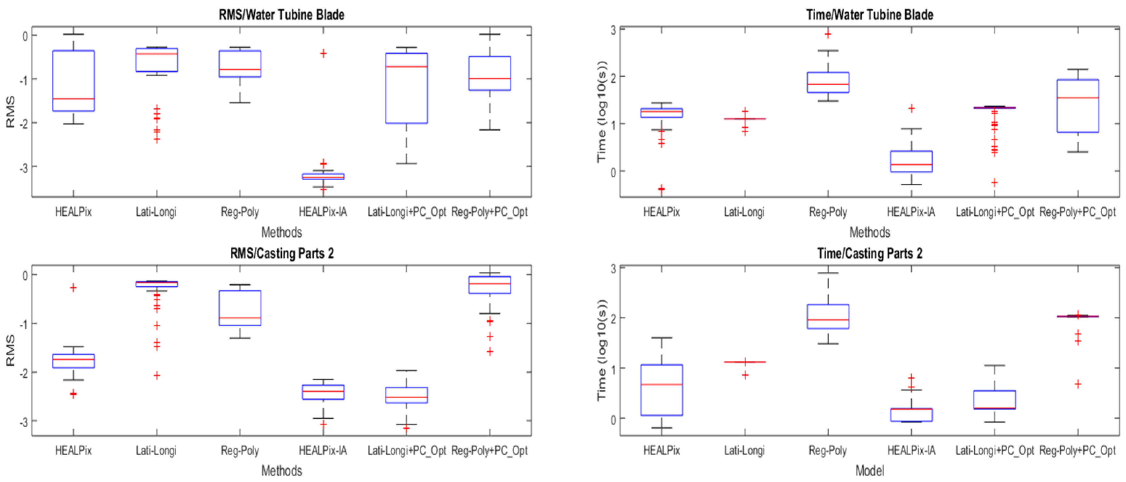
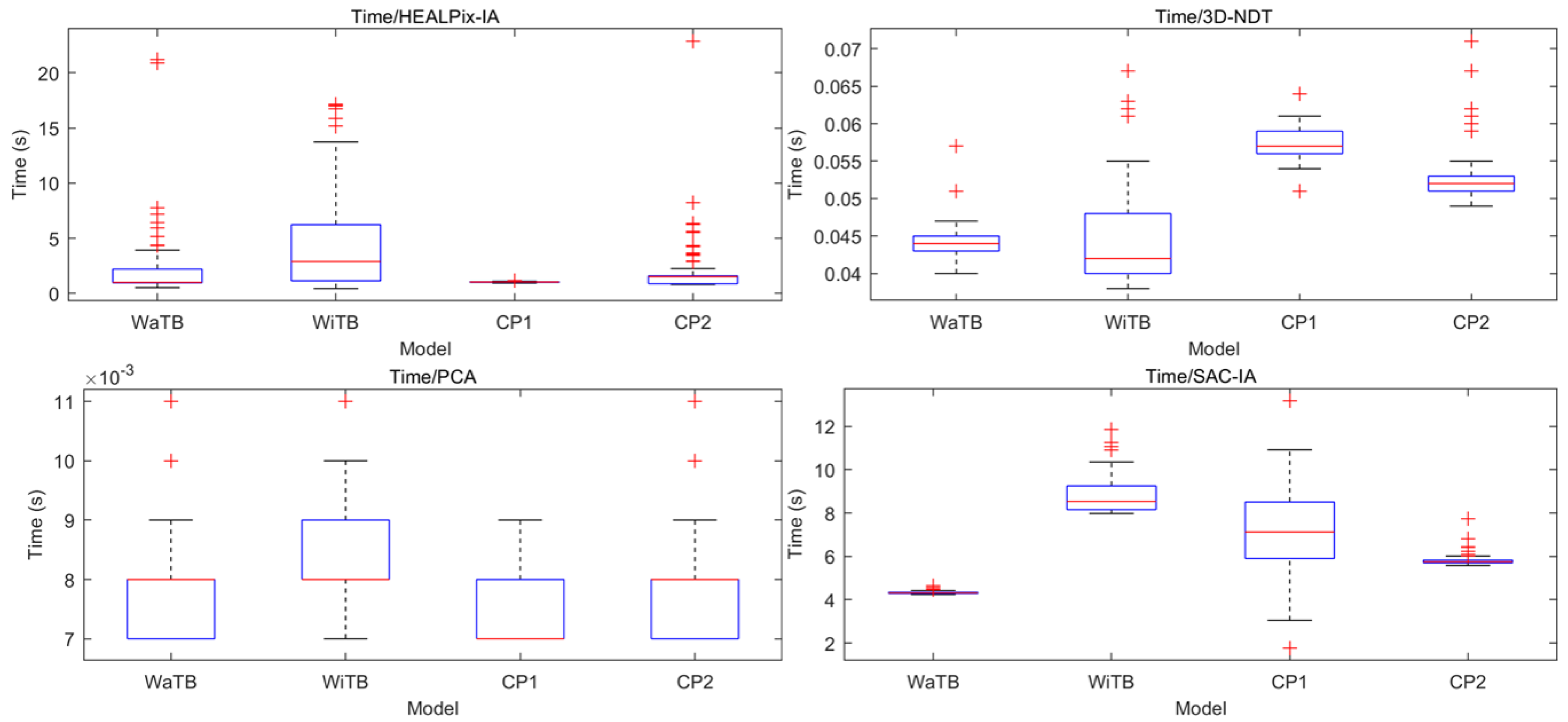
5.1.2. Compared with Other Rough Registration Methods
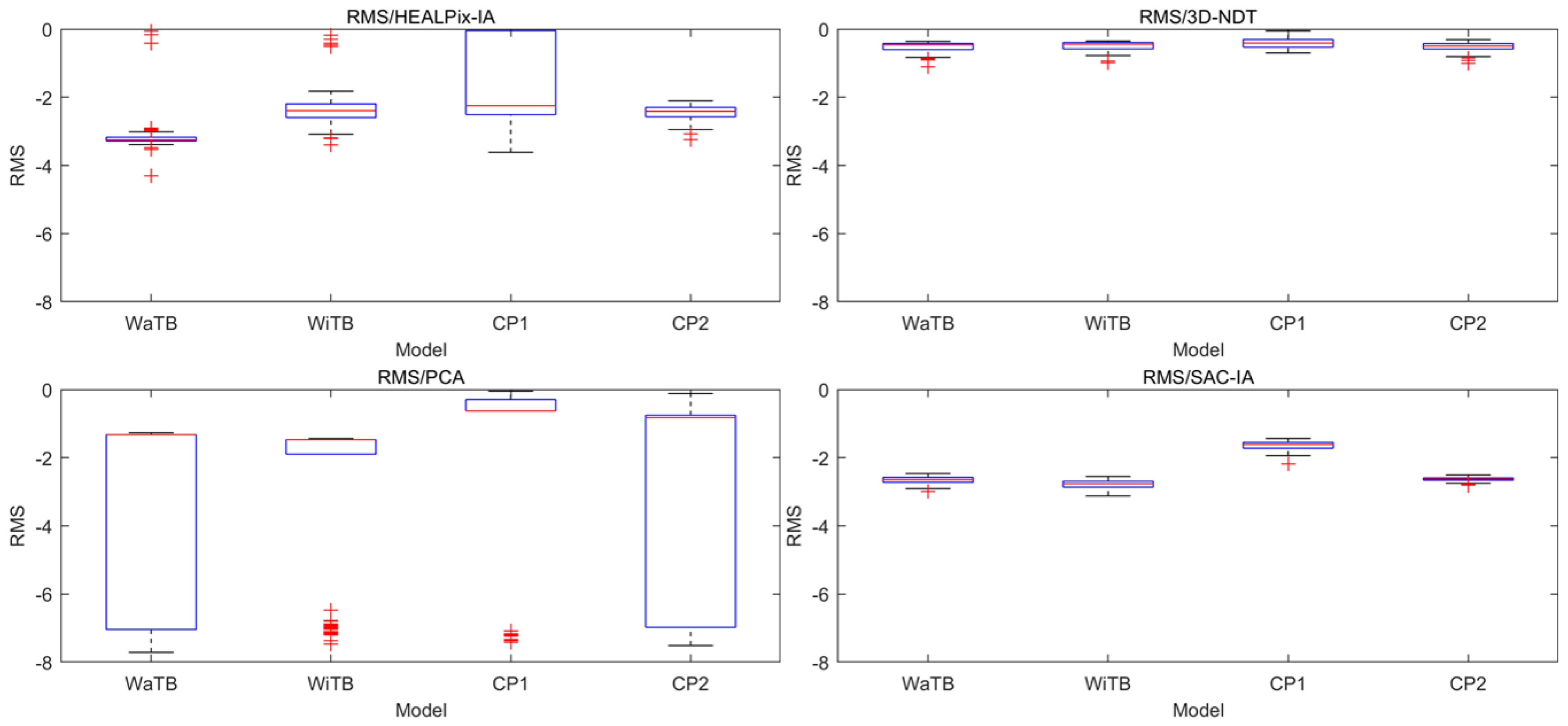
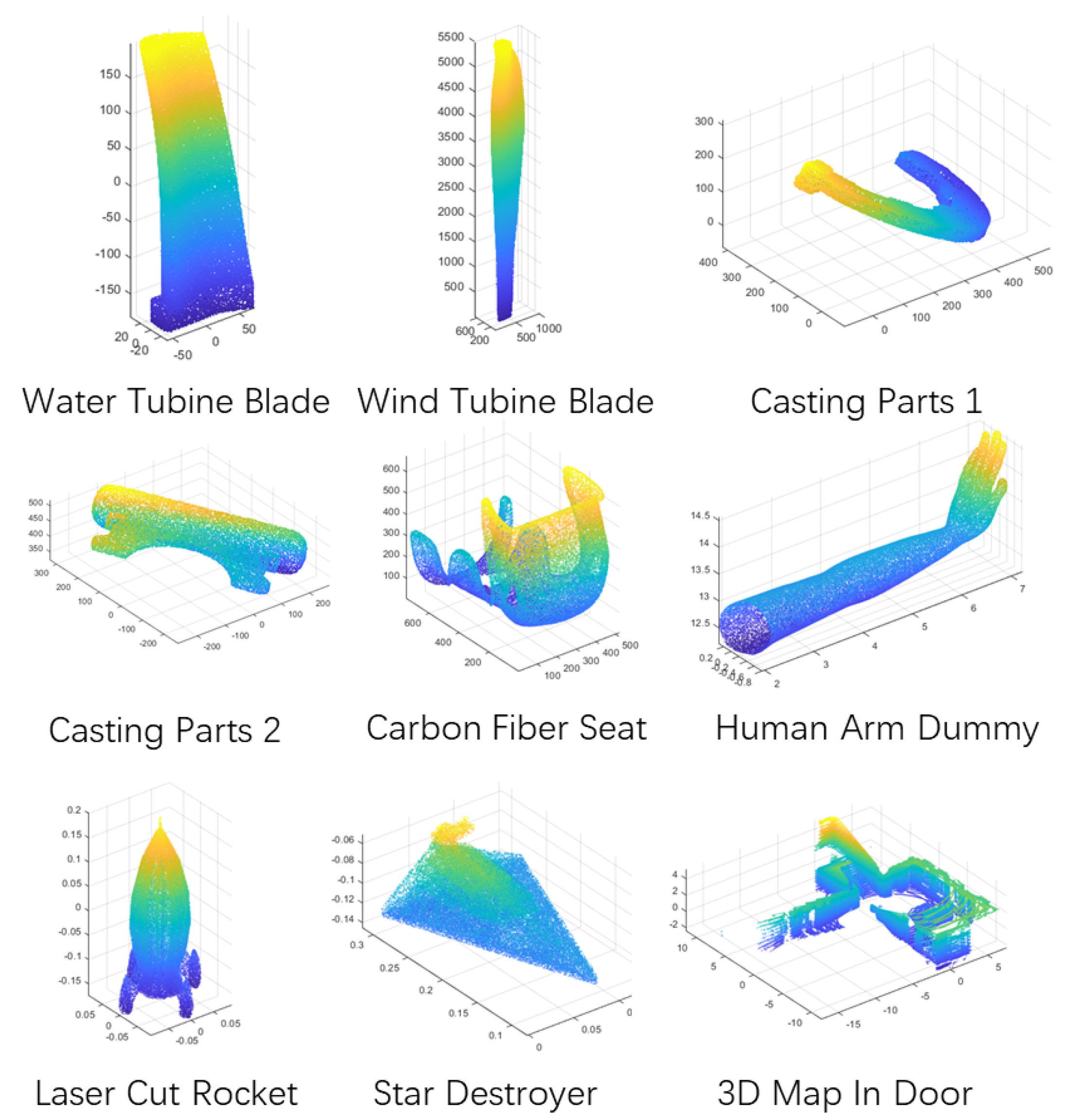
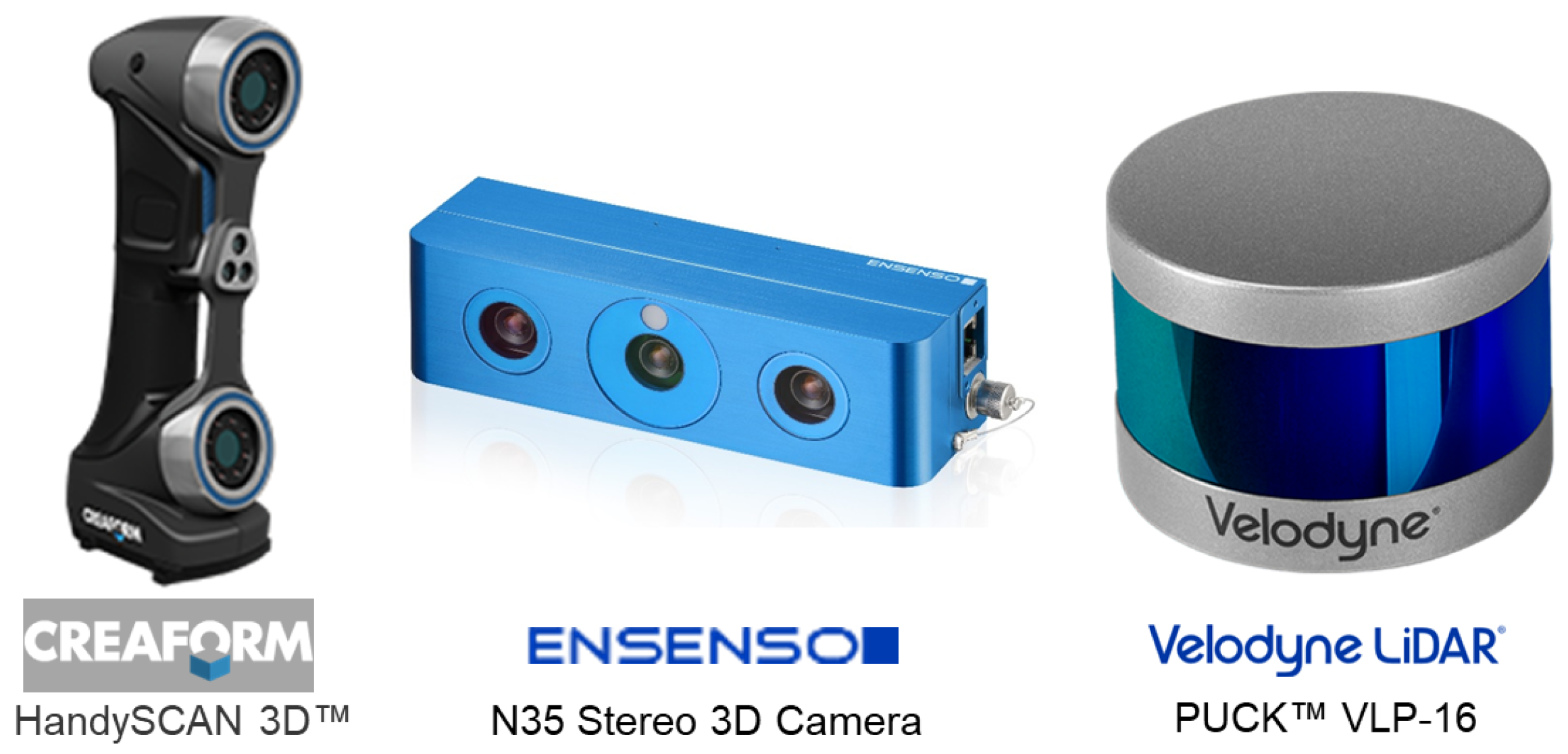
5.1.3. Tests on Real Data with Different Features via Various Sensors
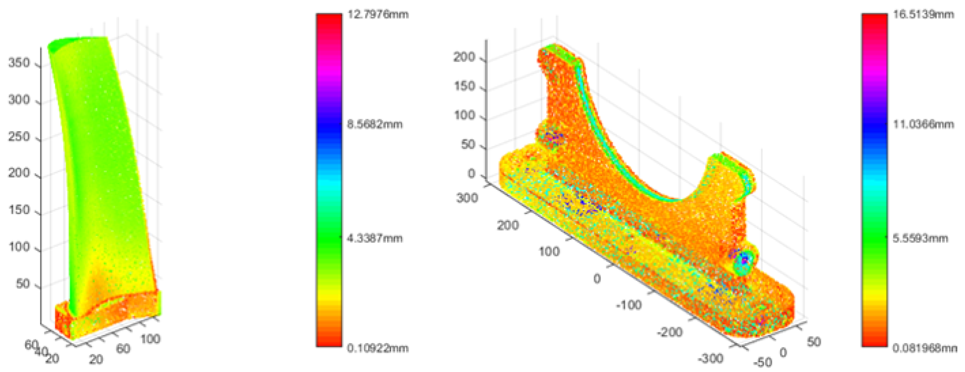
5.2. MA Analysis Test
6. Conclusions
Author Contributions
Funding
Conflicts of Interest
Abbreviations
| ICP | Iterative Closest Point |
| EGI | Extended Gaussian Image |
| SLAM | Simultaneous Localization And Mapping |
| MA | Machining Allowance |
| CMM | coordinate measuring machine |
| PCA | principal component analysis |
| FPFH | Fast Point Feature Histograms |
| Sac-IA | Sample Consensus-Initial Alignment |
| NDT | Normal Distributions Transform |
| RMS | Root Mean Square distances |
References
- Balsa-Barreiro, J.; Avariento, J.P.; Lerma, J.L. Airborne light detection and ranging (LiDAR) point density analysis. Sci. Res. Essays 2012, 7, 3010–3019. [Google Scholar] [CrossRef]
- Choi, C.; Taguchi, Y.; Tuzel, O.; Liu, M.Y.; Ramalingam, S. Voting-based pose estimation for robotic assembly using a 3D sensor. In Proceedings of the IEEE International Conference on Robotics and Automation, St. Paul, MN, USA, 14–18 May 2012; pp. 1724–1731. [Google Scholar]
- Holz, D.; Behnke, S. Sancta Simplicitas—On the efficiency and achievable results of SLAM using ICP-based incremental registration. In Proceedings of the 2010 International Conference on Robotics and Automation, Anchorage, AK, USA, 4–8 May 2010; pp. 1380–1387. [Google Scholar]
- Miao, S.; Zhang, W.J.; Liao, R. A CNN regression approach for real-time 2D/3D registration. IEEE Trans. Med. Imaging 2016, 35, 1352–1363. [Google Scholar] [CrossRef] [PubMed]
- Li, Z.; Gou, J.; Chu, Y. Geometric algorithms for workpiece localization. IEEE Trans. Robot. Autom. 1998, 14, 864–878. [Google Scholar]
- Tan, G.; Zhang, L.; Liu, S.; Zhang, W. A fast and differentiated localization method for complex surfaces inspection. Int. J. Precis. Eng. Manuf. 2015, 16, 2631–2639. [Google Scholar] [CrossRef]
- Shanoer, M.M.; Abed, F.M. Evaluate 3D laser point clouds registration for cultural heritage documentation. Egypt. J. Remote Sens. Space Sci. 2018, 21, 295–304. [Google Scholar] [CrossRef]
- Balsa-Barreiro, J.; Fritsch, D. Generation of visually aesthetic and detailed 3D models of historical cities by using laser scanning and digital photogrammetry. Digit. Appl. Archaeol. Cult. Herit. 2018, 8, 57–64. [Google Scholar] [CrossRef]
- Owda, A.; Balsa-Barreiro, J.; Fritsch, D. Methodology for digital preservation of the cultural and patrimonial heritage: Generation of a 3D model of the Church St. Peter and Paul (Calw, Germany) by using laser scanning and digital photogrammetry. Sens. Rev. 2018, 38, 282–288. [Google Scholar] [CrossRef]
- Lague, D.; Brodu, N.; Leroux, J. Accurate 3D comparison of complex topography with terrestrial laser scanner: Application to the Rangitikei canyon (N-Z). ISPRS J. Photogramm. Remote Sens. 2013, 82, 10–26. [Google Scholar] [CrossRef]
- Chu, Y.X.; Gou, J.B.; Li, Z.X. On the Hybrid Workpiece Localization/Envelopment Problem. IEEE Int. Conf. Robot. Autom. 1998, 4, 1–25. [Google Scholar]
- Gou, J.B.; Chu, Y.X.; Xiong, Z.H.; Li, Z.X. A Geometric Method for Computation of Datum Reference Frames. IEEE Trans. Robot. Autom. 2000, 16, 797–806. [Google Scholar] [CrossRef]
- Li, X.; Li, W.; Jiang, H.; Zhao, H. Automatic evaluation of machining allowance of precision castings based on plane features from 3D point cloud. Comput. Ind. 2013, 64, 1129–1137. [Google Scholar] [CrossRef]
- Wang, H.; Zhou, M.X.; Zheng, W.Z.; Shi, Z.B.; Li, H.W. 3D machining allowance analysis method for the large thin-walled aerospace component. Int. J. Precis. Eng. Manuf. 2017, 18, 399–406. [Google Scholar] [CrossRef]
- Sun, Y.W.; Xu, J.T.; Guo, D.M.; Jia, Z.Y. A unified localization approach for machining allowance optimization of complex curved surfaces. Precis. Eng. 2009, 33, 516–523. [Google Scholar] [CrossRef]
- Rusu, R.B.; Blodow, N.; Beetz, M. Fast Point Feature Histograms (FPFH) for 3D registration. In Proceedings of the 2009 IEEE International Conference on Robotics and Automation, Kobe, Japan, 12–17 May 2009; pp. 3212–3217. [Google Scholar]
- Weingarten, J.; Gruener, G.; Siegwart, R. A Fast and Robust 3D Feature Extraction Algorithm for Structured Environment Reconstruction; EPFL Scientific Publications: Geneva, Switzerland, 2003; pp. 1–6. [Google Scholar]
- Prasad, G. Segmentation of 3D MR Images of the Brain Using a PCA Atlas and Nonrigid Registration; University of California: Los Angeles, CA, USA, 2010; pp. 1–63. [Google Scholar]
- Schneider, D.C.; Eisert, P. Automatic and robust semantic registration of 3D head scans. In Proceedings of the 5th European Conference on Visual Media Production, London, UK, 26–27 November 2008. [Google Scholar] [CrossRef]
- Magnusson, M. The Three-Dimensional Normal-Distributions Transform—An Efficient Representation for Registration, Surface Analysis, and Loop Detection. Ph.D. Thesis, Örebro University, Örebro, Sweden, 2009. [Google Scholar]
- Makadia, A.A.; Patterson, V.; Daniilidis, K. Fully automatic registration of 3D point clouds. In Proceedings of the IEEE Computer Society Conference on Computer Vision and Pattern Recognition, New York, NY, USA, 17–22 June 2006; pp. 1297–1304. [Google Scholar]
- Dold, C. Extended Gaussian images for the registration of terrestrial scan data. In Proceedings of the ISPRS Workshop “Laser Scanning 2005”, Enschede, The Netherlands, 12–14 September 2005; pp. 180–185. [Google Scholar]
- Kang, S.B.; Ikeuchi, K. The Complex EGI: A New Representation for 3-D Pose Determination. IEEE Trans. Pattern Anal. Mach. Intell. 1993, 15, 707–721. [Google Scholar] [CrossRef]
- Hilaga, M.; Shinagawa, Y.; Kohmura, T.; Kunii, T.L. Topology matching for fully automatic similarity estimation of 3D shapes. In Proceedings of the 28th Annual Conference on Computer Graphics and Interactive Techniques—SIGGRAPH’01, Los Angeles, CA, USA, 12–17 August 2001; pp. 203–212. [Google Scholar]
- Hu, Z.; Chung, R.; Fung, K.S. EC-EGI: Enriched complex EGI for 3D shape registration. Mach. Vis. Appl. 2010, 21, 177–188. [Google Scholar] [CrossRef]
- Ezra, E.; Sharir, M.; Efrat, A. On the performance of the ICP algorithm. Comput. Geom. 2008, 41, 77–93. [Google Scholar] [CrossRef]
- Huizinga, W.; Poot, D.H.; Guyader, J.M.; Klaassen, R.; Coolen, B.F.; Van Kranenburg, M.; Van Geuns, R.J.; Uitterdijk, A.; Polfliet, M.; Vandemeulebroucke, J.; et al. PCA-based groupwise image registration for quantitative MRI. Med. Image Anal. 2016, 29, 65–78. [Google Scholar] [CrossRef] [PubMed]
- Sasatani, S.; Han, X.H.; Chen, Y.W. Image Registration Using PCA And Gradient Method For Super-resolution Imaging. In Proceedings of the 2nd International Conference on Software Engineering and Data Mining, Chengdu, China, 23–25 June 2010; pp. 631–634. [Google Scholar]
- Zhan, Y.; Yin, J. Robust local tangent space alignment via iterative weighted PCA. Neurocomputing 2011, 74, 1985–1993. [Google Scholar] [CrossRef]
- Rusu, R.B.; Blodow, N.; Marton, Z.C.; Beetz, M. Aligning point cloud views using persistent feature histograms. In Proceedings of the 2008 IEEE/RSJ International Conference on Intelligent Robots and Systems, Nice, France, 22–26 September 2008; pp. 3384–3391. [Google Scholar]
- Magnusson, M.; Duckett, T. A Comparison of 3D Registration Algorithms for Autonomous Underground Mining Vehicles. In Proceedings of the European Conference on Mobile Robotics (ECMR 2005), Ancona, Italy, 7–10 September 2005; pp. 86–91. [Google Scholar]
- Tsin, Y.; Kanade, T. A Correlation-Based Approach to Robust Point Set Registration. In European Conference on Computer Vision; Springer: Berlin/Heidelberg, Germany, 2004. [Google Scholar]
- Straub, J.; Campbell, T.; How, J.P.; Fisher, J.W. Efficient global point cloud alignment using Bayesian nonparametric mixtures. In Proceedings of the 30th IEEE Conference on Computer Vision and Pattern Recognition—CVPR 2017, Honolulu, HI, USA, 21–26 July 2017; pp. 2403–2412. [Google Scholar]
- Ahuja, S.; Waslander, S.L. 3D scan registration using curvelet features. In Proceedings of the Conference on Computer and Robot Vision—CRV 2014, Montréal, QC, Canada, 7–9 May 2014; pp. 77–83. [Google Scholar]
- Calabretta, M.R.; Roukema, B.F. Mapping on the HEALPix grid. Mon. Not. R. Astron. Soc. 2007, 381, 865–872. [Google Scholar] [CrossRef]


| Model (Abbreviation) | Features | Sensors |
|---|---|---|
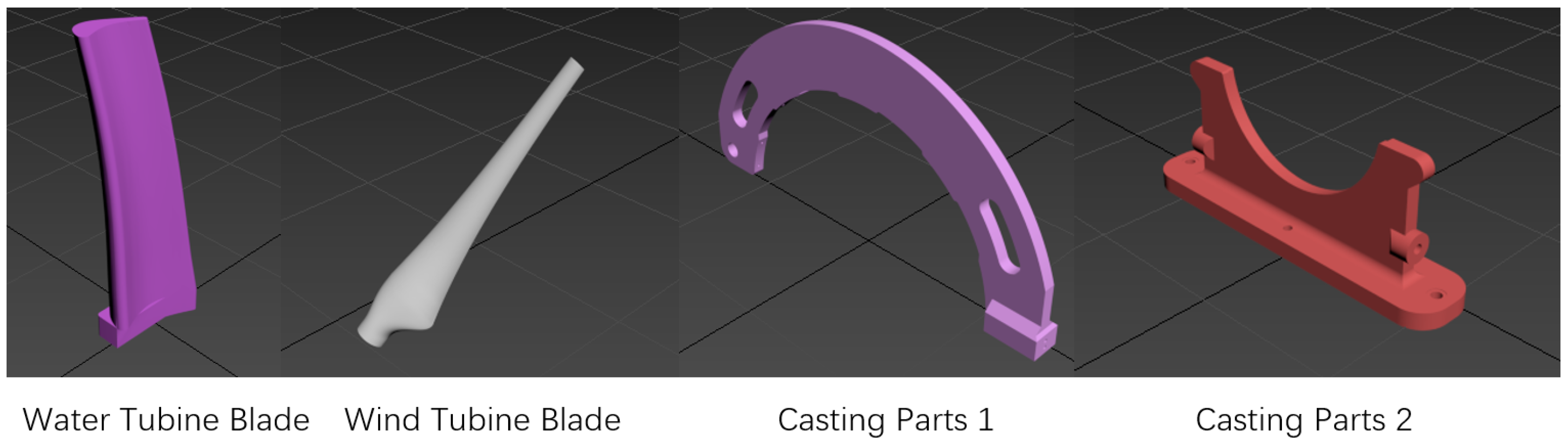
| Water Turbine Blade (WaTB) | complex Curve Surface | 3D laser scanner |
| Wind Turbine Blade (WiTB) | complex curve Surface | 3D laser scanner |
| Casting Parts 1 (CP1) | thin-walled, large plane | 3D laser scanner |
| Casting Parts 2 (CP2) | mirror symmetry | 3D laser scanner |
| Carbon Fiber Seat (CFS) | thin-walled, curve surface | 3D laser scanner |
| Human Arm Dummy (HAD) | unstructureed features | 3D laser scanner |
| Laser Cut Rocket (LCR) | rotational symmetry | 3D laser scanner |
| Star Destroyer (SD) | mirror symmetry | 3D Camera |
| 3D Map In Door (Map) | low dense data | 3D LiDAR |
| Models and Criteria | Sac-IA | HEALPix-IA | |
|---|---|---|---|
| WaTB-RMS | Ave | 2.9 × 10⁻² | 3.4 × 10⁻³ |
| Var | 8.1 × 10⁻⁴ | 4.9 × 10⁻⁵ | |
| WaTB-time (ms) | Ave | 4932.1 | 3830.8 |
| Var | 6.3 × 10³ | 2.7 × 10⁴ | |
| WaTB-opt time (ms) | Ave | 7222.7 | 10,110.5 |
| Var | 1.6 × 10⁷ | 2.2 × 10⁷ | |
| CP2-RMS | Ave | 1.2 × 10⁻² | 7.2 × 10⁻³ |
| Var | 3.5 × 10⁻⁵ | 1.1 × 10⁻⁶ | |
| CP2-time (ms) | Ave | 5953.2 | 4818.3 |
| Var | 8.7 × 10³ | 4.5 × 10³ | |
| CP2-opt time (ms) | Ave | 9049.9 | 8066.5 |
| Var | 2.65 × 10⁷ | 1.4 × 10⁷ |
© 2019 by the authors. Licensee MDPI, Basel, Switzerland. This article is an open access article distributed under the terms and conditions of the Creative Commons Attribution (CC BY) license (http://creativecommons.org/licenses/by/4.0/).
Share and Cite
Gao, Y.; Du, Z.; Xu, W.; Li, M.; Dong, W. HEALPix-IA: A Global Registration Algorithm for Initial Alignment. Sensors 2019, 19, 427. https://doi.org/10.3390/s19020427
Gao Y, Du Z, Xu W, Li M, Dong W. HEALPix-IA: A Global Registration Algorithm for Initial Alignment. Sensors. 2019; 19(2):427. https://doi.org/10.3390/s19020427
Chicago/Turabian StyleGao, Yongzhuo, Zhijiang Du, Wei Xu, Mingyang Li, and Wei Dong. 2019. "HEALPix-IA: A Global Registration Algorithm for Initial Alignment" Sensors 19, no. 2: 427. https://doi.org/10.3390/s19020427
APA StyleGao, Y., Du, Z., Xu, W., Li, M., & Dong, W. (2019). HEALPix-IA: A Global Registration Algorithm for Initial Alignment. Sensors, 19(2), 427. https://doi.org/10.3390/s19020427