SWIR AOTF Imaging Spectrometer Based on Single-pixel Imaging


Abstract
1. Introduction
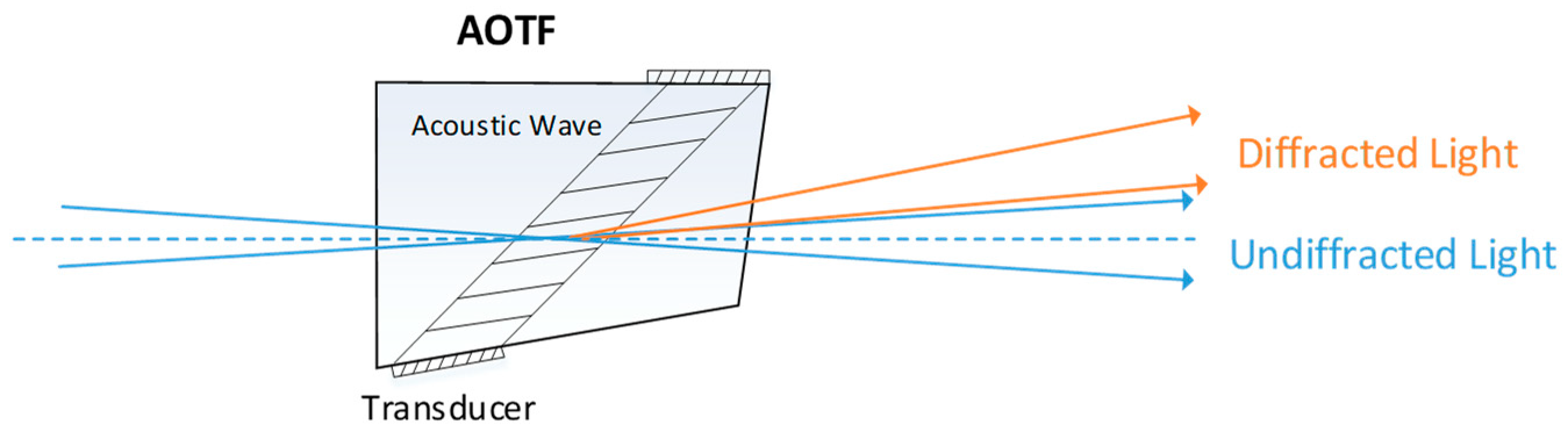
2. Background
3. Method
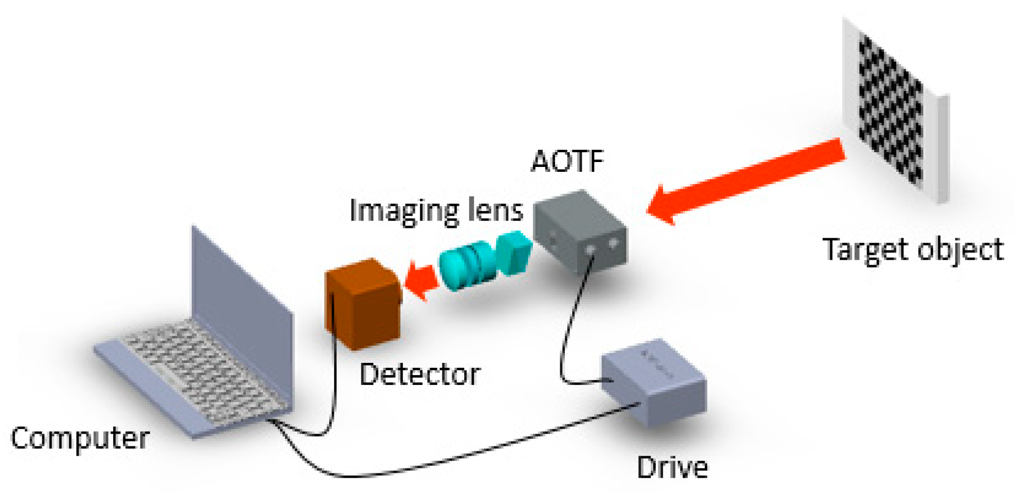
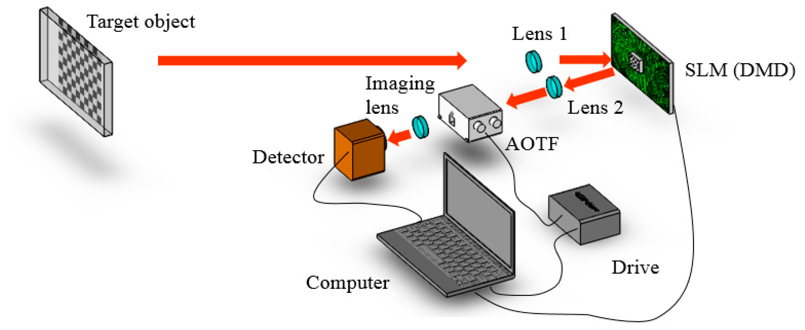
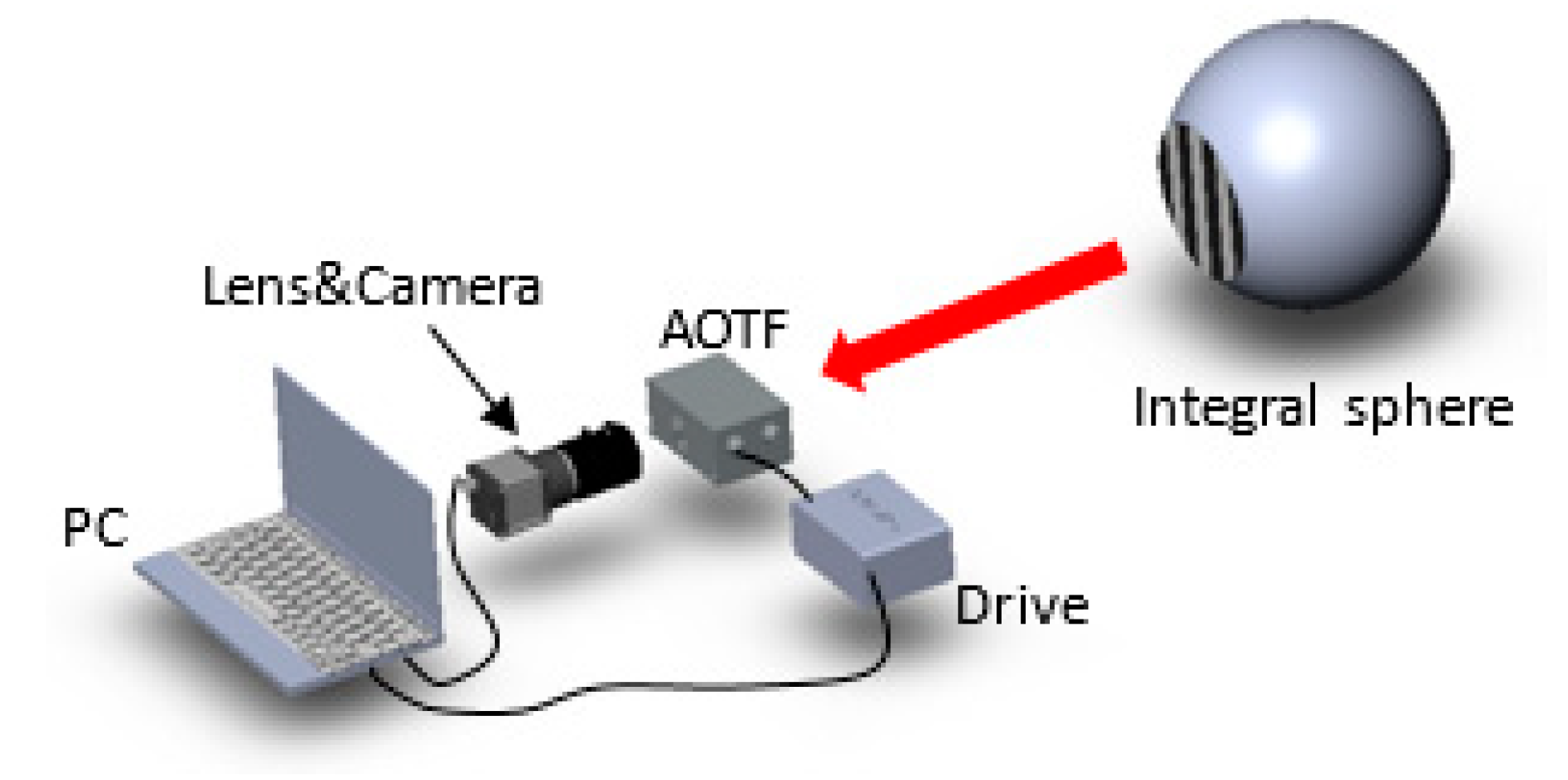
3.1. Setup of the AOTF Imaging Spectrometer Based on SPI
3.2. Principle of SPI with a Hadamard Mask Pattern
3.3. Process of Grabbing Spectral Images
4. Experiments and Results
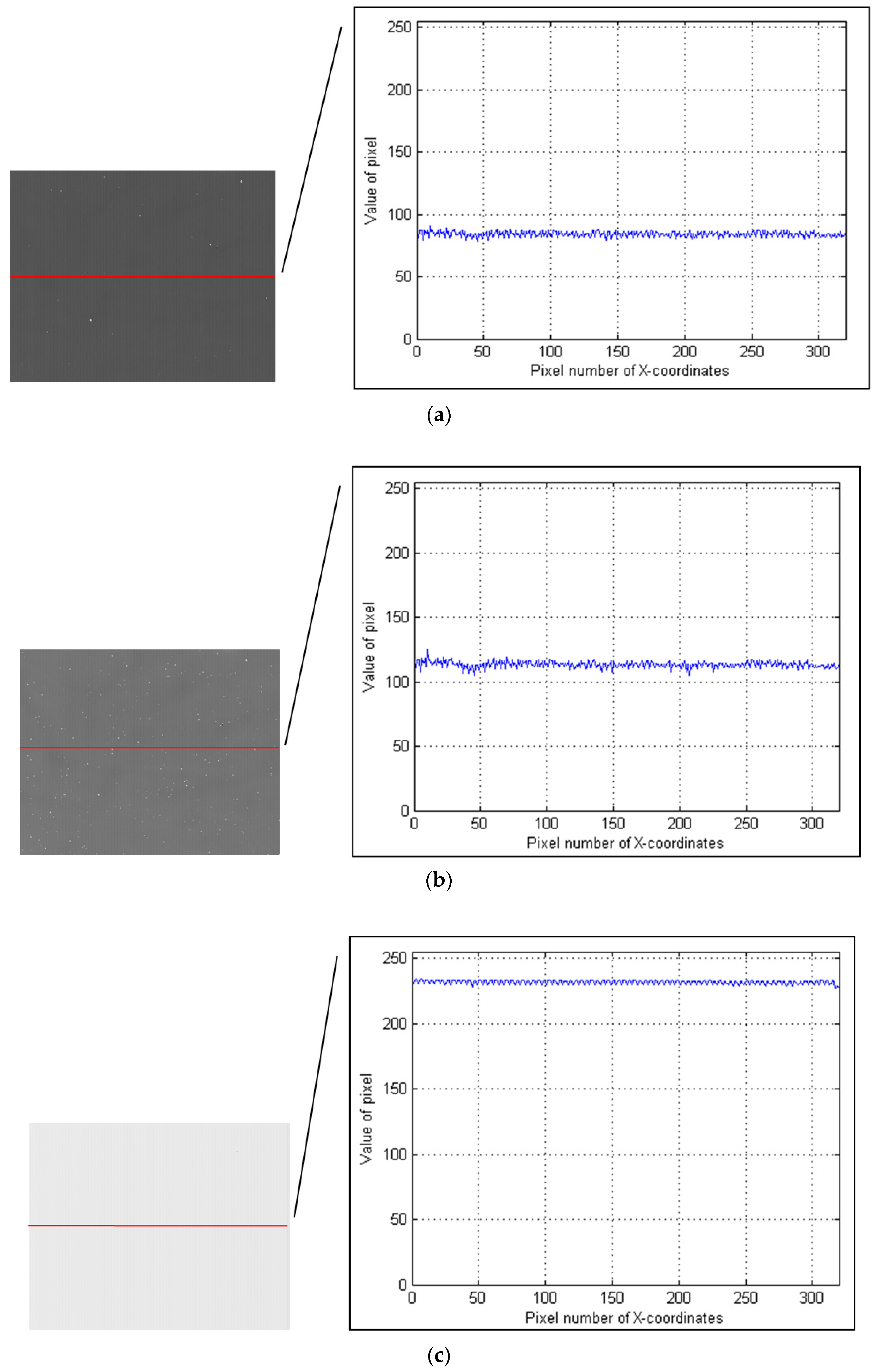
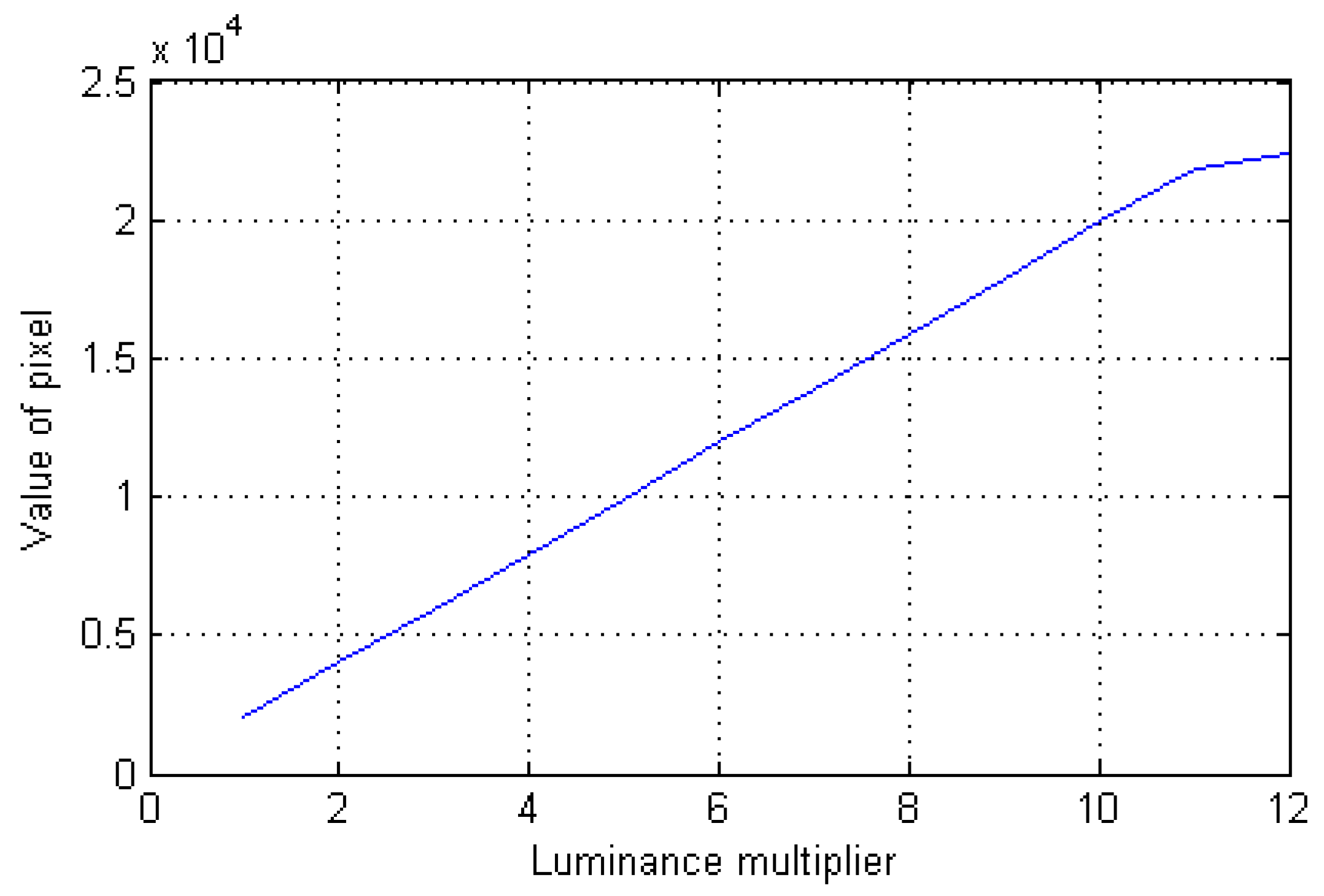
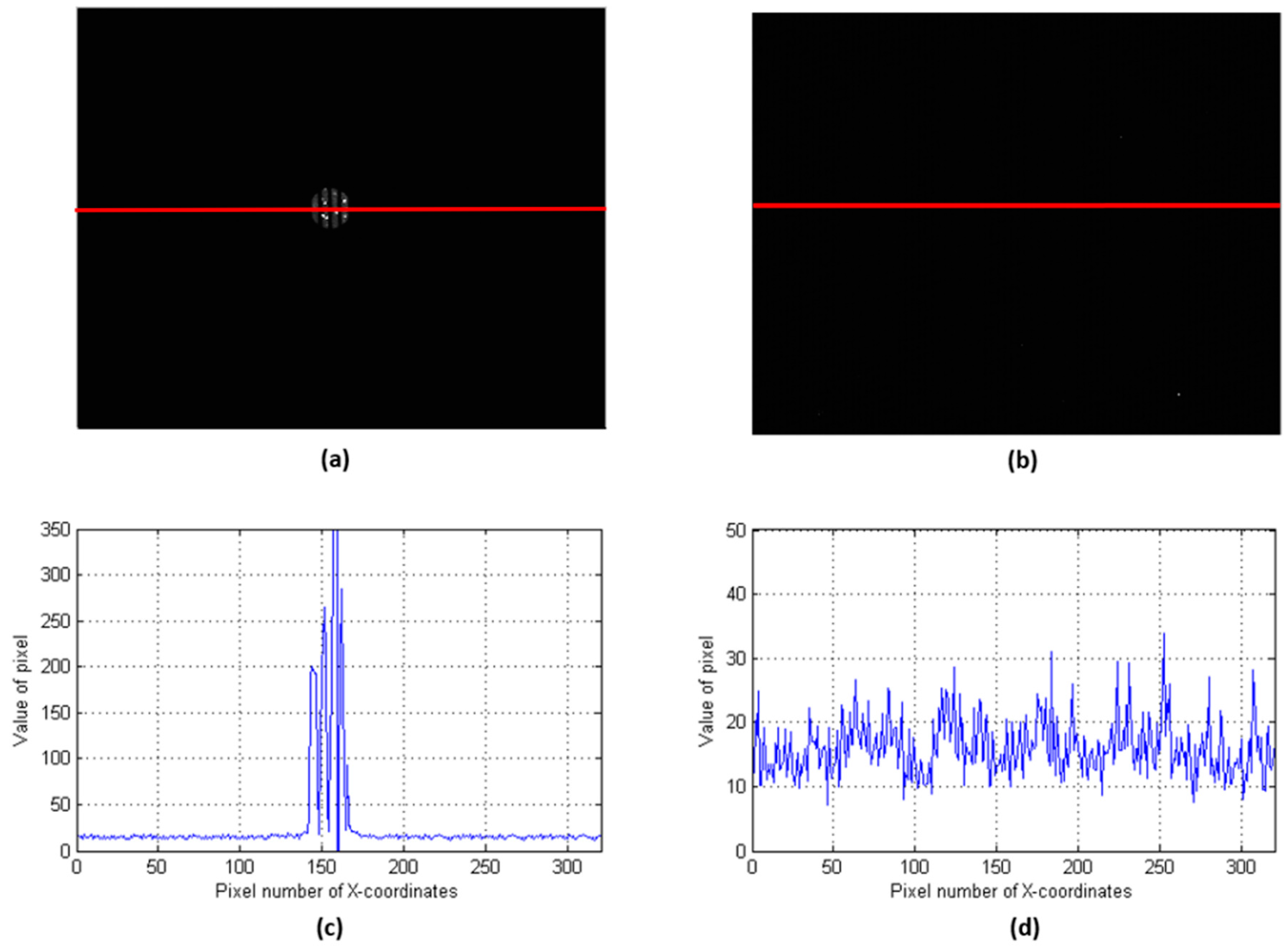
4.1. Camera Response Contrast between Long-focus Lens (Lens of the Traditional System) and Short-Focus Lens (Lens of the SPI System)
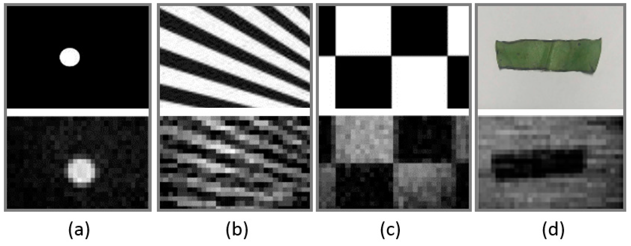
4.2. SPI Imaging Spectrometer and Results of Different Objects
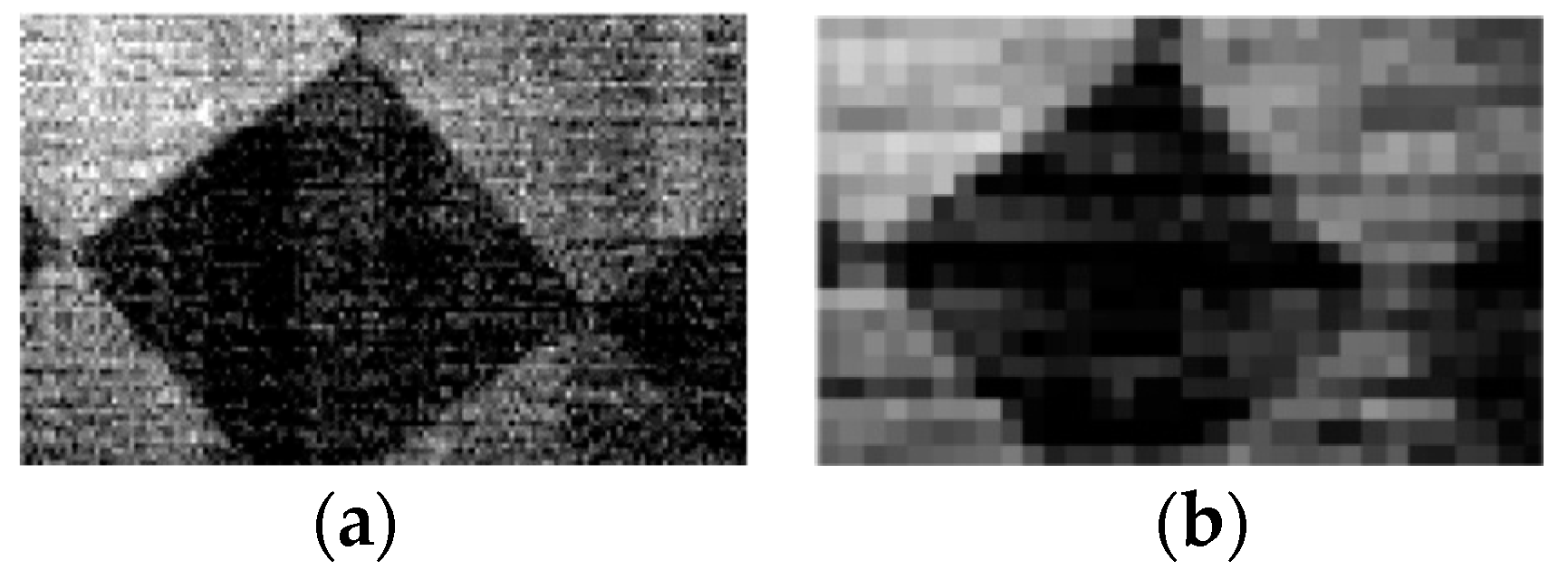
4.3. High- and Low-Resolution Images
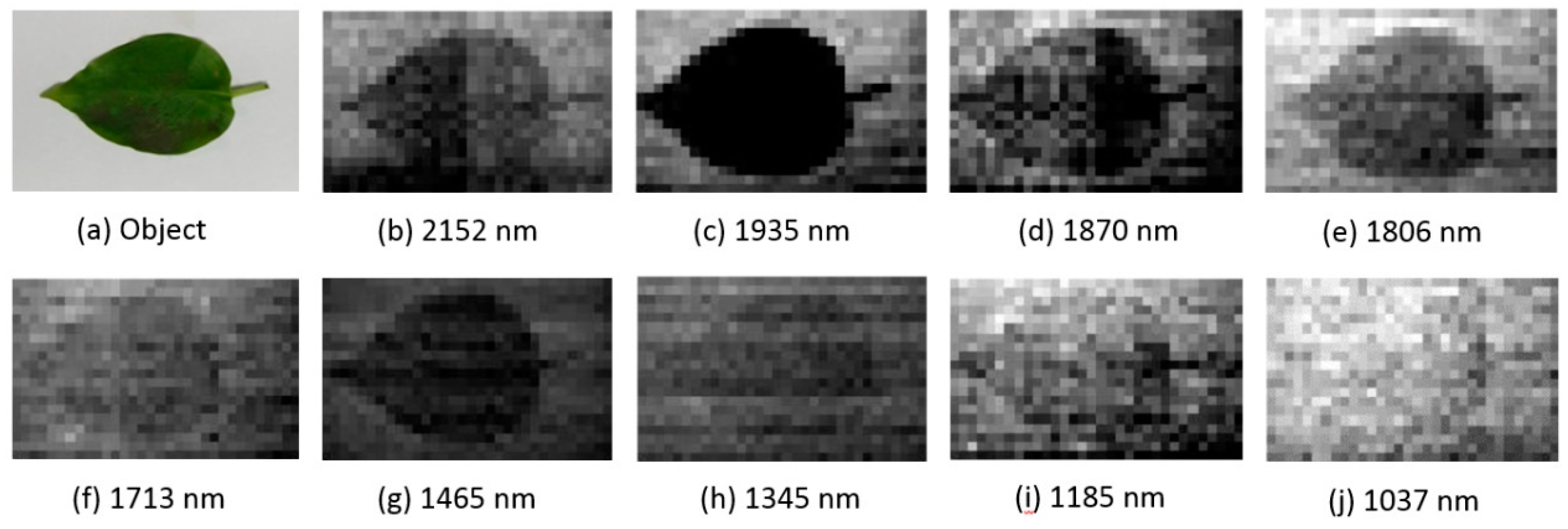
4.4. Images of Different Bands
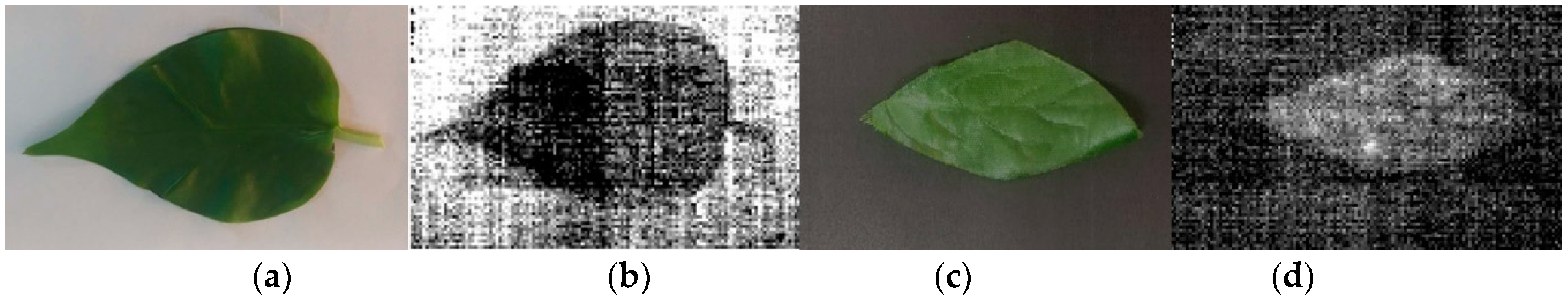
4.5. Experiment between Real and Fake Plants
5. Discussions and Conclusions
Author Contributions
Funding
Conflicts of Interest
References
- Harris, S.E.; Wallace, R.W. Acousto-optic tunable filter. J. Opt. Soc. Am. 1969, 59, 744–747. [Google Scholar] [CrossRef]
- Chang, I.C. Noncollinear acousto-optic tunable filter with large angular aperture. Appl. Phys. Lett. 1974, 25, 370–372. [Google Scholar] [CrossRef]
- Yano, T.; Watanable, A. Acoustooptic TeO2 tunable filter using far-off-axis anisotropic Bragg diffraction. Appl. Opt. 1976, 15, 2250–2258. [Google Scholar] [CrossRef] [PubMed]
- Glenar, D.A.; Blaney, D.L.; Hillman, J.J. AIMS: Acousto-optic imaging spectrometer for spectral mapping of solid surfaces. Acta Astronaut. 2003, 52, 389–396. [Google Scholar] [CrossRef]
- Dekemper, E.; Fussen, D.; Van Opstal, B.; Vanhamel, J.; Pieroux, D.; Vanhellemont, F.; Mateshvili, N.; Franssens, G.; Voloshinov, V.; Janssen, C.; et al. ALTIUS: A spaceborne AOTF-based UV-VIS-NIR hyperspectral imager for atmospheric remote sensing. Proc. SPIE 2014, 9241, 92410L. [Google Scholar]
- He, Z.P.; Wang, B.Y.; Lv, G.; Li, C.L.; Yuan, L.Y.; Xu, R.; Chen, K.; Wang, J.Y. Visible and near-infrared imaging spectrometer and its preliminary results from the Change 3 project. Rev. Sci. Instrum. 2014, 85, 13–18. [Google Scholar] [CrossRef]
- Calpe-Maravilla, J.; Vila-Frances, J.; Ribes-Gomez, E.; Duran-Bosch, V.; Munoz-Mari, J.; Amoros-Lopez, J.; Gomez-Chova, L.; Tajahuerce-Romera, E. 400– to 1000–nm imaging spectrometer based on acousto-optic tunable filters. J. Electron. Imaging 2006, 15, 023001. [Google Scholar] [CrossRef]
- Cirilli, M.; Bellincontro, A.; Urbani, S.; Servili, M.; Esposto, S.; Mencarelli, F.; Muleo, R. On-field monitoring of fruit ripening evolution and quality parameters in olive mutants using a portable NIR-AOTF device. Food Chem. 2016, 199, 96–104. [Google Scholar] [CrossRef]
- Dekemper, E.; Vanhamel, J.; Opstal, B.V.; Fussen, D. The AOTF-based NO2 camera. Atmos. Meas. Technol. 2016, 9, 6025–6034. [Google Scholar] [CrossRef]
- Ward, J.; Farries, M.; Pannell, C.; Wachman, E. An acousto-optic based hyperspectral imaging camera for security and defence applications. Proc. SPIE 2010, 7835, 78350U. [Google Scholar] [CrossRef]
- Valle, S.; Ward, J.; Pannell, C.; Johnson, N.P. Acousto-optic tunable filter for imaging application with high performance in the IR region. Proc. SPIE 2015, 9359, 93590E. [Google Scholar] [CrossRef]
- Sizov, F.F. Infrared detectors: Outlook and means’, Semiconductors Physics. Quantum Electron. Opto-Electron. 2000, 3, 52–58. [Google Scholar]
- Rogalski, A.; Chrzanowski, K. Infrared devices and techniques. Opto-Electron. Rev 2002, 10, 111–136. [Google Scholar]
- Chorier, P.; Tribolet, P.M.; Fillon, P.; Manissadjian, A. Application needs and trade-offs for short-wave infrared detectors. Proc. SPIE 2003, 5074, 363–373. [Google Scholar]
- Gupta, N. Performance characterization of VNIR and SWIR spectropolarimetric imagers. Proc. SPIE 2015, 9482, 948216. [Google Scholar]
- Zhang, H.; Li, S.; Bao, M.; Wen, Q.; Wang, W.; Yan, H.; Zhang, X.; Wang, Z.; Wang, R. Research and development of AOTF based NIR spectrometer. Proc. SPIE 2010, 7655, 76552V. [Google Scholar]
- Tawalbeh, R.; Voelz, D.G.; Glenar, D.A.; Xiao, X.; Chanover, N.J.; Hull, R.; Kuehn, D. Infrared acousto-optic tunable filter point spectrometer for detection of organics on mineral surfaces. Opt. Eng. 2013, 52, 063604. [Google Scholar] [CrossRef]
- Duarte, M.F.; Davenport, M.A.; Takhar, D.; Laska, J.N.; Sun, T.; Kelly, K.F.; Baraniuk, R.G. Single-Pixel Imaging via Compressive Sampling. IEEE Signal Process. Mag. 2008, 25, 83–91. [Google Scholar] [CrossRef]
- Soldevila, F.; Irles, E.; Durán, V.; Clemente, P.; Fernández-Alonso, M.; Tajahuerce, E.; Lancis, J. Single-pixel polarimetric imaging spectrometer by compressive sensing. Appl. Phys. B 2013, 113, 551–558. [Google Scholar] [CrossRef]
- Magalhães, F.; Araújo, F.M.; Correia, M.V.; Abolbashari, M.; Farahi, F. Active illumination single-pixel camera based on compressive sensing. Appl. Opt. 2011, 50, 405–414. [Google Scholar] [CrossRef]
- Gibson, G.M.; Sun, B.; Edgar, M.P.; Phillips, D.B.; Hempler, N.; Maker, G.T.; Malcolm, G.P.; Padgett, M.J. Real-time imaging of methane gas leaks using a single-pixel camera. Opt. Express 2017, 25, 2998–3005. [Google Scholar] [CrossRef] [PubMed]
- Welsh, S.S.; Edgar, M.P.; Bowman, R.; Jonathan, P.; Sun, B.; Padgett, M.J. Fast full-color computational imaging with single-pixel detectors. Opt. Express 2013, 21, 23068–23074. [Google Scholar] [CrossRef] [PubMed]
- Yan, Y.; Dai, H.; Liu, X.; He, W.; Chen, Q.; Gu, G. Colored adaptive compressed imaging with a single photodiode. Appl. Opt. 2016, 55, 3711–3718. [Google Scholar] [CrossRef] [PubMed]
- Salvador-Balaguer, E.; Clemente, P.; Tajahuerce, E.; Pla, F.; Lancis, J. Full-color stereoscopic imaging with a single-pixel photodetector. J. Display Technol. 2016, 12, 417–422. [Google Scholar] [CrossRef]
- Liu, B.L.; Yang, Z.H.; Liu, X.; Wu, L.A. Coloured computational imaging with single-pixel detectors based on a 2D discrete cosine transform. J. Mod. Opt. 2017, 64, 259–264. [Google Scholar] [CrossRef]
- Jin, S.; Hui, W.; Wang, Y.; Huang, K.; Shi, Q.; Ying, C.; Liu, D.; Ye, Q.; Zhou, W.; Tian, J. Hyperspectral imaging using the single-pixel Fourier transform technique. Sci. Rep. 2017, 7, 45209. [Google Scholar] [CrossRef] [PubMed]
- Bian, L.; Suo, J.; Situ, G.; Li, Z.; Fan, J.; Chen, F.; Dai, Q. Multispectral imaging using a single bucket detector. Sci. Rep. 2016, 6, 24752. [Google Scholar] [CrossRef]
- Zhang, Z.; Wang, X.; Zheng, G.; Zhong, J. Hadamard single-pixel imaging versus Fourier single-pixel imaging. Opt. Express 2017, 25, 19619–19639. [Google Scholar] [CrossRef]
- Ferri, F.; Magatti, D.; Lugiato, L.A.; Gatti, A. Differential ghost imaging. Phys. Rev. Lett. 2010, 105, 219902. [Google Scholar] [CrossRef]


| Specification of the AOTF | |
| Optical aperture | 10 mm × 10 mm |
| Spectral range | 900–2500 nm |
| Spectral resolution | 5–20 nm |
| Acceptance angle | 6–10° |
| Separation angle | 7.1–7.8° |
| Specification of the DMD | |
| Wavelength range | 700–2500 nm |
| Pattern rate, 8-bit (max) | 120 Hz |
| Micromirror array size | 912 × 1140 |
| Micromirror pitch | 7.6 µm |
© 2019 by the authors. Licensee MDPI, Basel, Switzerland. This article is an open access article distributed under the terms and conditions of the Creative Commons Attribution (CC BY) license (http://creativecommons.org/licenses/by/4.0/).
Share and Cite
Zhao, H.; Xu, Z.; Jiang, H.; Jia, G. SWIR AOTF Imaging Spectrometer Based on Single-pixel Imaging. Sensors 2019, 19, 390. https://doi.org/10.3390/s19020390
Zhao H, Xu Z, Jiang H, Jia G. SWIR AOTF Imaging Spectrometer Based on Single-pixel Imaging. Sensors. 2019; 19(2):390. https://doi.org/10.3390/s19020390
Chicago/Turabian StyleZhao, Huijie, Zefu Xu, Hongzhi Jiang, and Guorui Jia. 2019. "SWIR AOTF Imaging Spectrometer Based on Single-pixel Imaging" Sensors 19, no. 2: 390. https://doi.org/10.3390/s19020390
APA StyleZhao, H., Xu, Z., Jiang, H., & Jia, G. (2019). SWIR AOTF Imaging Spectrometer Based on Single-pixel Imaging. Sensors, 19(2), 390. https://doi.org/10.3390/s19020390