1. Introduction
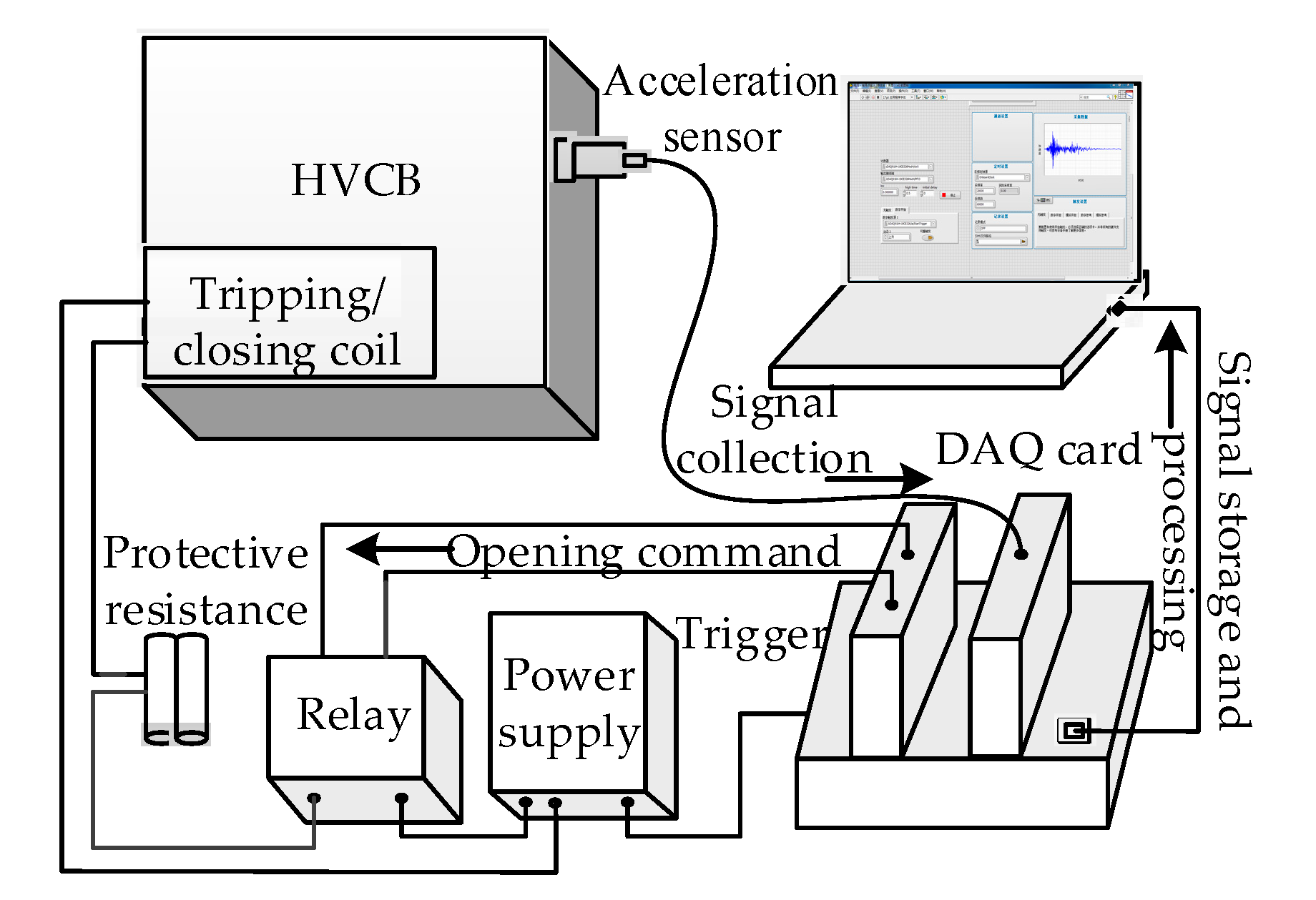
High-voltage circuit breakers (HVCBs) are the most important control and primary protection equipment in electric power systems [
1,
2]. The operation states of HVCBs are directly related to the stability and reliability of the power system. The analysis object of HVCBs mainly operates via the moving contact travel-time characteristic method, the tripping (closing) coil current method, and the vibration signal method at present [
3,
4,
5,
6]. The operating mechanism is the main factor affecting the reliability of circuit breakers. There are many mechanical failures, such as a lack of spring energy storage, and screw loosening by vibration signals [
7]. Therefore, HVCBs fault diagnoses based on vibration signals is of great significance [
8]. The analysis process mainly includes signal processing, feature extraction, and fault diagnosis.
Due to the non-stationary and the nonlinear characteristics of the vibration signals of HVCBs, traditional signal processing methods analyze the vibration signal in the time domain and frequency domain, and extract time–frequency domain features. The commonly used signal processing methods are empirical mode decomposition (EMD) [
9,
10], ensemble empirical mode decomposition (EEMD) [
11], and local mean decomposition (LMD) [
12], etc. The above methods have achieved good fault diagnosis results, but there are still some shortcomings. Feature extractions with EMD and LMD have some problems in the process of decomposition, such as mode mixing and end effects [
11]. Although EEMD has suppressed mode mixing by adding white noise, the method also increases the amount of computation and decomposes many components beyond the real composition of the signal [
12]. At the same time, the process of the signal processing method is complex, with high time complexity, which improves the computational cost and the industrialization difficulty of the related technologies.
The features of the traditional vibration signals include time domain features, frequency domain features, and time-frequency features. The existing features set can accurately describe the different state of the fault signals. However, the features of HVCBs vibration signals are widely distributed in the frequency and time domains, and it is difficult to extract effective features from the specific frequency domain or the time domain, which are affected by the specific installation environment in the actual work [
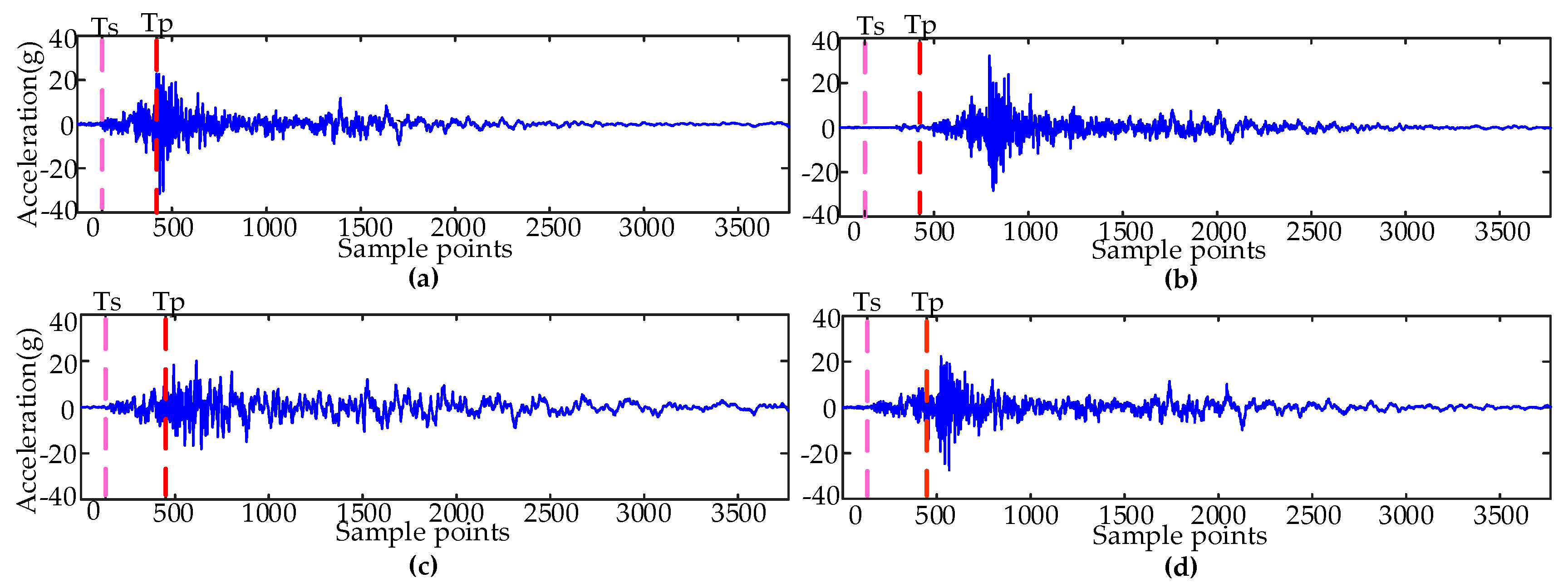
13]. Because of the differences in the degree of attenuation and starting time of the different types of fault vibration signals, HVCBs failure states can be analyzed by the time domain features when directly extracted from the original vibration signal. The features are extracted by calculating the mean, variance, and standard deviation by different time domain segmentation scales from the original signal [
13,
14,
15,
16]. By extracting the abundant original signal features, the fault information can be described in detail. However, the dimensions of the feature set will be increased, and redundant features may be included in the feature set. The feature set with high dimensional features will affect the fault diagnosis accuracy and efficiency of the classifier. Therefore, selecting the optimal feature subset from higher-dimensional features extracted from original signals is the key to improve the efficiency and accuracy of HVCBs fault diagnosis.
Fault diagnosis methods for circuit breakers include support vector machine (SVM) [
17], neural networks (NNs) [
7], etc. However, there are many kinds of mechanical faults in HVCBs, and the operation of HVCBs is rare. Furthermore, the cost of obtaining the fault sample experiment is high. It is difficult to acquire enough fault samples with all fault types. Traditional multi-classifiers are easily identify the fault type data without training samples as the known or normal states. The effect of condition monitoring is seriously affected.
To improve the efficiency of feature extraction of vibration signals, and to avoid untrained samples of unknown type faults from being identified as normal or error known types, a new method of mechanical fault diagnosis for HVCBs based on feature extraction and selection without signal processing is proposed. Firstly, the vibration signals of the HVCBs are segmented by a time scale that starts collecting standard normal vibration signals. Secondly, time–domain features are extracted from each part of the divided signal and used to construct the feature vector. The sequential forward selection method with the regulated Fisher’s criterion (RFC) index is used to determine the optimal feature subset, based on Gini importance. Finally, the optimal subset construction of the hierarchical hybrid classifier is based on the one-class support vector machine (OCSVM) and random forest (RF) for state recognition. The effectiveness of the new method is verified by the measured signal.
2. Feature Importance and Fault Classifiers
2.1. Gini Importance
The Gini importance is used to measure the node impurity, and it can be used to measure the feature importance [
18]. Suppose that
S is a dataset containing
s samples, which can be divided into
n classes.
is the number of samples contained in class
a. The Gini index of the set is:
where
, which is used to expressed the probability of any sample belonging to class
a.
When RF uses a feature to divide nodes, it can divide
S into
m subsets, denoted with
, The Gini index of split
S is:
where
is the samples number in subset
.
It is known from Equation (3) that the higher the Gini importance, the better the feature division [
18].
2.2. Random Forest
RF is composed of a series of classification and regression tree (CART) models
, and voting by multiple decision trees, where
is a classification model for CART,
X is an input feature vector,
is a random vector that follows the independent and identical distribution, and
l represents the number of the classifier. For a given independent variable
X, the optimal classification is achieved by aggregating the voting results of each CART. The detailed classification principle of RF can be found in [
19,
20,
21], and the basic classification process is as follows:
- (1)
q samples are randomly extracted from the original set Q, to constitute a self-help sample set, repeated l times.
- (2)
During the training process, random selection from the feature space M is a candidate feature of non-leaf node splitting, and the nodes are divided with each candidate feature, and the best segmentation feature is chosen as the segmentation feature of the node. This process is repeated until all of the non-leaf nodes of each tree are classified, and the training process is then ended.
- (3)
Determining the optimal classification results by the majority voting method of each of the classification results.
The optimum ranges of the minimum leaf number
and the candidate feature number
for each node are
and
. The value of
is set to 10, and
is the dimension of the feature subset. RF integrates the characteristics of bagging and random selection feature splitting; its advantages are: (1) out-of-bag (OOB) data generated by the bagging method, and it can be used to measure the importance of a single variable and estimate the generalization error of the combined classifier models; (2) Due to the large number theorem, with the increase of decision tree in RF, it is not easy to be over-fitted; (3) The algorithm can tolerate abnormal values and noises properly, and it has high classification accuracy [
22].
2.3. One-Class Support Vector Machine (OCSVM)
OCSVM only uses normal samples to complete the training process and to determine the mechanical state of the device. The speed of the training and decision is fast, and the anti-noise performance is good. It is suitable for the field of mechanical condition monitoring with high reliability.
Suppose there is a sample ; mapping it to a high-dimensional feature space through the kernel function , it has better aggregation and it can solve an optimal hyperplane in the feature space, so as to achieve the maximum separation between the target data, and the origin of the coordinates. The decision function is ; it attempts to separate the training set from the origin, and maximize the distance between the hyperplane and the origin.
The weight
of the support vector and the threshold
can be described by solving the following quadratic programming problem:
where
is used to control the proportion of support vectors in the training samples. After introducing the kernel function, the above problem can be transformed into a dual problem:
In OCSVM,
is a determined threshold, determining the separation hyperplane with the weight vector
, through the decision equation, OCSVM can determine whether the sample z is a fault sample [
17].
2.4. Construction of the Hierarchical Classifier
Because the types of fault samples are not comprehensive, there are some unknown types of faults occurring in practical work. When an unknown type of fault occurs, by using multi-class classifier to identify HVCBs mechanical faults, the unknown faults will be identified as a known fault or normal. Although OCSVM can accurately monitor the state of mechanical failure, it cannot identify the type of fault as known or unknown. Therefore, a hybrid classifier is constructed with OCSVM and RF. Using OCSVM to avoid mistaken identifications of fault status, we further identified the unknown fault types accurately without training samples, through RF and OCSVM.
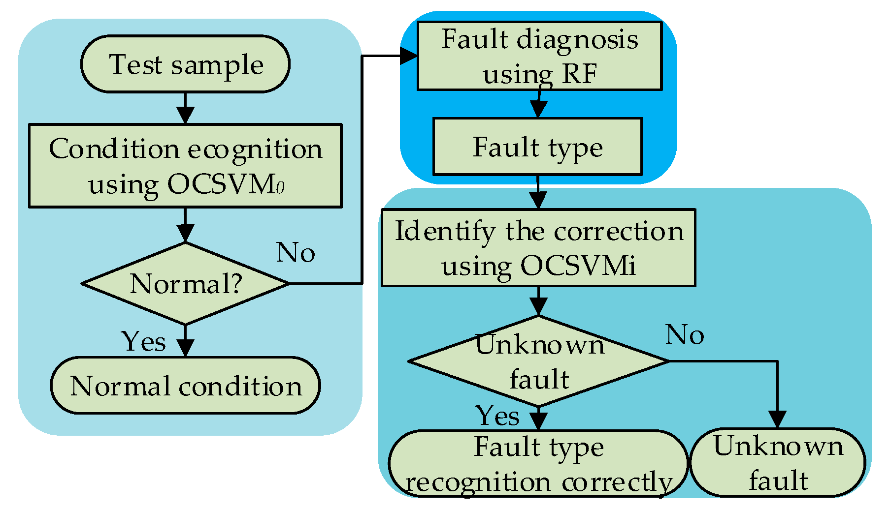
Figure 1 is a flowchart of fault diagnosis based on a hybrid classifier. Firstly, the OCSVM
0 classifier is applied to identify the normal and fault states of HVCB. If the HVCB is in a fault condition, RF is used to identify the specific fault types. Then, aiming at the fault condition identified by RF, OCSVM
l (where
l is a three-fault condition) is used to identify and correct the condition, based on the OCSVM
l model trained by a specific known fault type.
4. Comparison of Classification Effects of Different Feature Extraction Methods
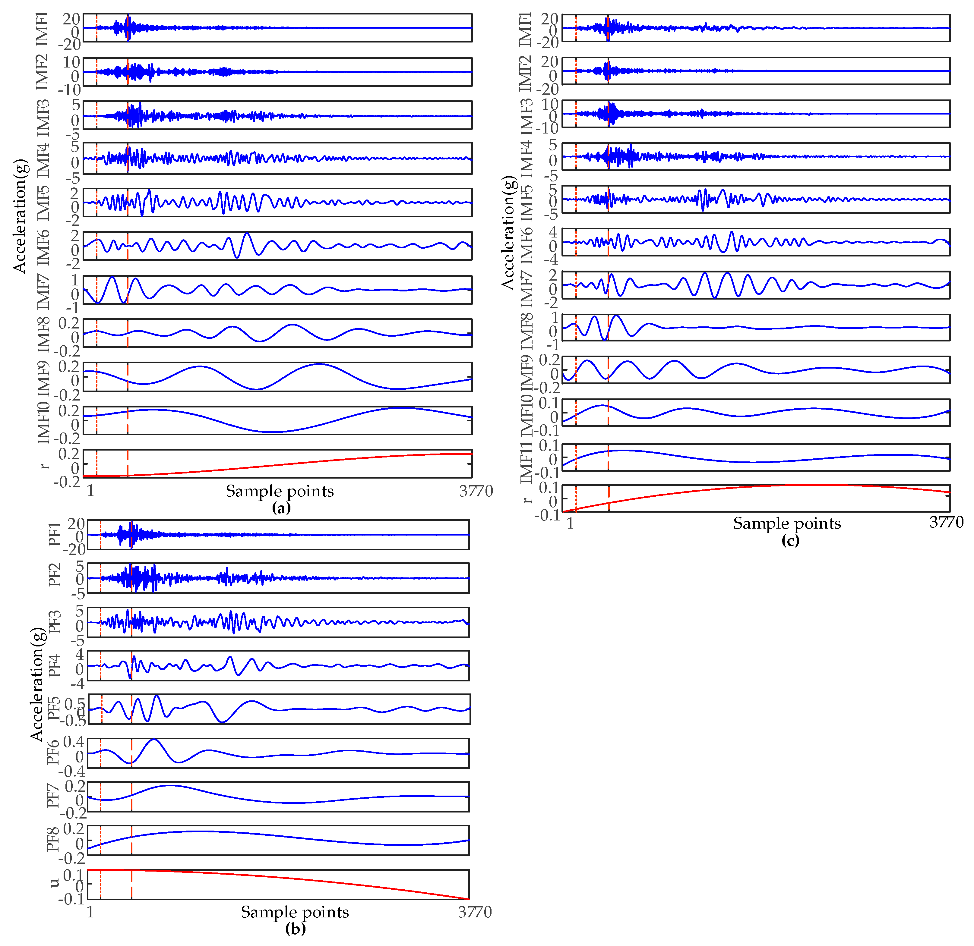
In order to compare the effects of feature extraction in a new method, three signal processing methods of EMD, EEMD, and LMD were used to extract features, to compare them with the new method.
Figure 4 is the result of signal decomposition and time domain segmentation by using EMD, EEMD, and LMD. The time domain segmentation scale was the same as the new method. EMD and EEMD decompose the signal into some intrinsic mode functions (IMFs). LMD decomposes the signal into multiple product functions (PFs) with instantaneous frequency.
When using different feature extraction methods,
Table 3 shows the recognition accuracy without unknown types when using multiple classifiers and the original feature set dimension.
Di is the features dimension, and
Ac is the accuracy of the condition recognition.
As shown in
Table 3, when the new method divided the signal into 29 segments and nine segments, the new method could identify three states effectively, while the traditional signal processing method had mistaken identifications. In this paper, the feature dimensions extracted by the new method were 153 and 493. Compared with the traditional signal method, the feature dimension was lower. Therefore, the new method feature extraction not only improved the accuracy of the state recognition, but also effectively reduced the complexity of the original feature set.
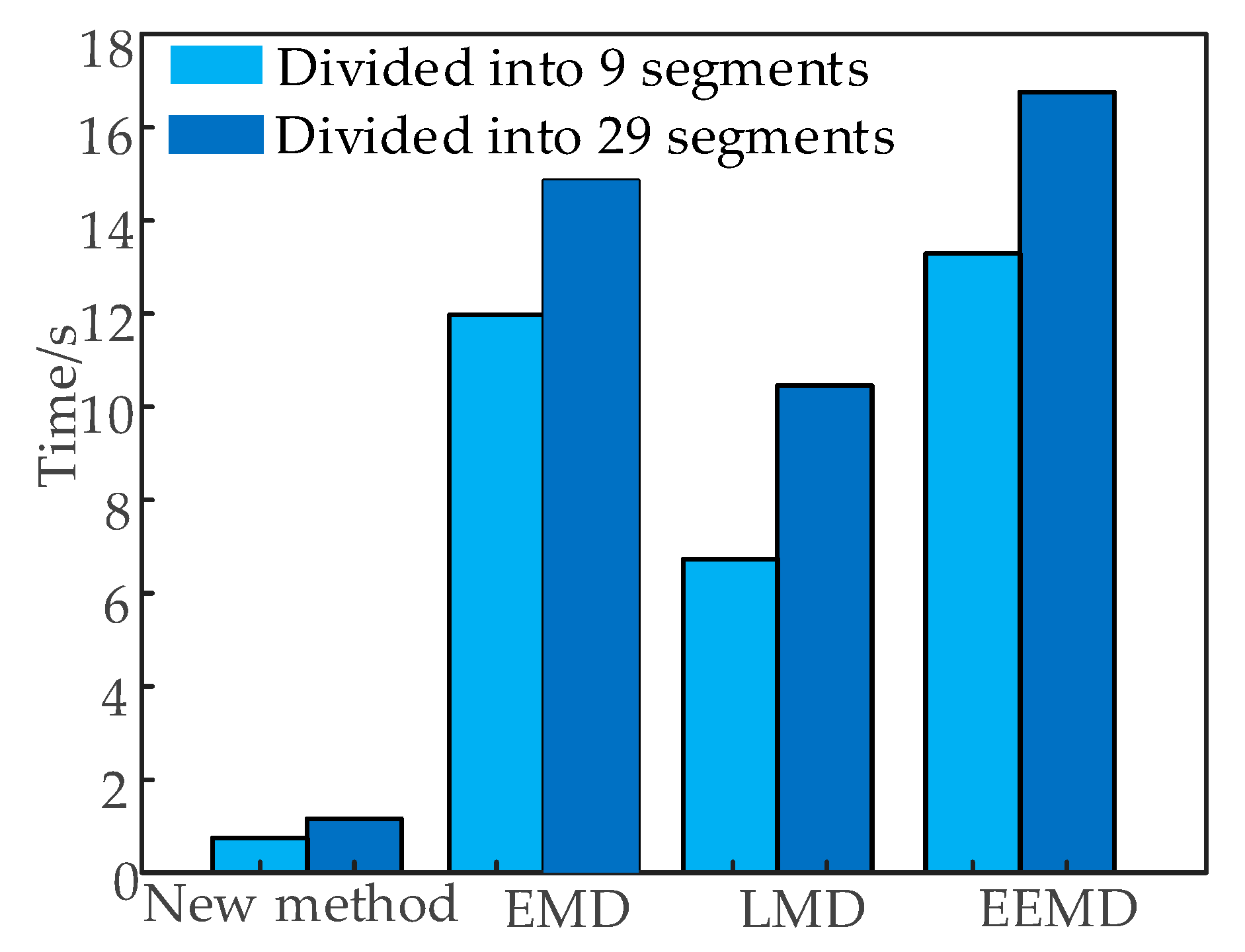
Figure 5 shows the time statistics for extracting features by direct time-domain segmentation and traditional signal processing methods. According to
Figure 5, no matter the time domain segmentation method that is used, the new method without signal processing removed the signal processing, and extracted the time-domain features only for a single time series of the original signal.
The computation time of the new method was lower than that of the traditional methods, which were needed to extract features from multiple IMF or PF time series. The efficiency of the feature extraction was higher than EMD, LMD, and EEMD. When the sampling rate of the vibration signal to be analyzed is higher, the advantages of the new method will be more obvious.
5. Feature Selection
In the existing feature selection, when the wrapper method was used; combined with the particle swarm algorithm, the feature subset satisfying the classification accuracy rate is found according to the classifier effect, but the efficiency of the optimization is low. In actual work, the filter method receives more applications. Experiments are carried out according to the statistical results of the features [
23,
24,
25].
RF is an ensemble learning method. Its Gini importance index takes the comprehensive contribution of features in different feature combinations into account, and analysis becomes more comprehensive. The features were in descending order according to the Gini importance, and SFS was carried out to obtain a better candidate feature set. After that, the classifier was constructed with different feature subsets, and the evaluation index of RFC was calculated. Finally, the best feature subset was determined, which was used to train the optimal classifier.
5.1. The Gini Importance of Time Domain Features
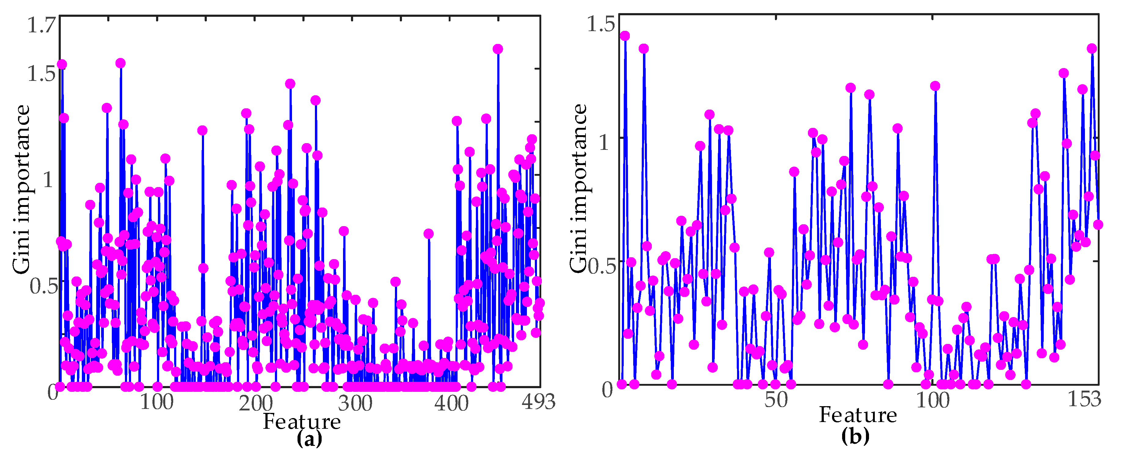
In order to reduce the complexity of the classifier, three classes of signals were used as the classification targets. The complete original feature set was used as the input feature vector to train the RF classifier, and all of the Gini importance were obtained. The importance of the original feature set constructed by two times domain segmentation methods is shown in
Figure 6. As is evident in
Figure 6, the Gini importance of the different features were quite different. Therefore, feature ordering could be carried out according to the Gini importance.
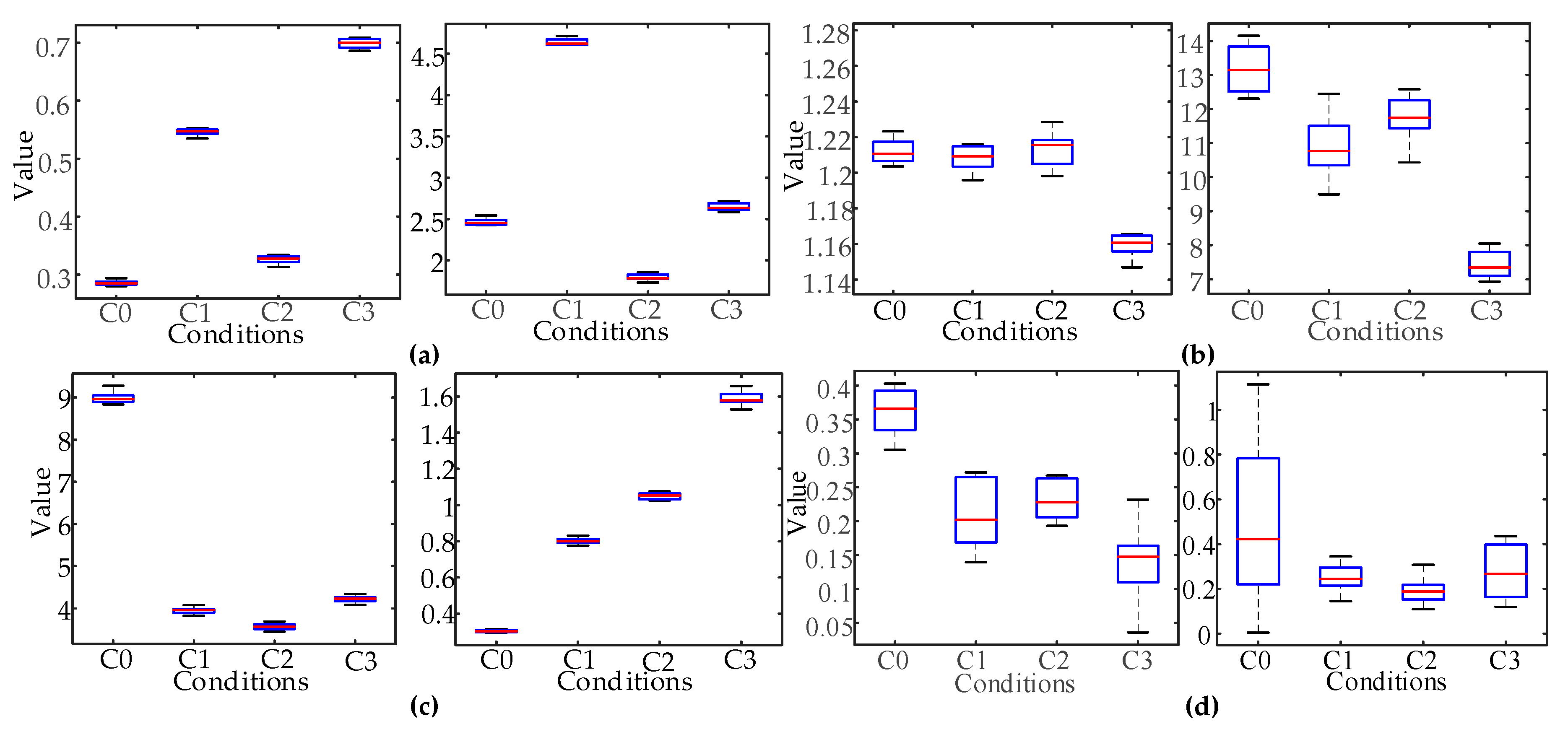
In order to prove the effectiveness of feature classification ability, based on Gini importance, Under two kinds of time domain segmentation scales, two groups were selected from the highest and lowest Gini importance of the features, respectively. A box plot was drawn to analyze the distribution of the features. According to the distribution of features, the classification ability of the features with different Gini importance was intuitively compared. According to the Gini importance, the best features of 29 segments are F450 and F62, and the worst features are F311 and F313; the best features of the nine segments are F31 and F34, and the worst features are F16 and F37.
As shown in
Figure 7, the box diagram distribution was determined by 10 groups of typical fault samples. The distribution of the features with high Gini importance was centralized with no crossing. The degree of distinction between the different classes was high. The distribution of the features with low Gini importance was wide and overlapped. The degree of distinction between the different classes was low. The validity of the feature classification ability was verified, based on Gini importance.
5.2. Sequential Forward Selection Based on RFC
In the process of sequential forward selection, the optimal feature subset was determined by the classification accuracy of the feature subset, and the JF index of RFC.
The separation of features could be determined by the Fisher criterion in pattern recognition [
25]:
Fisher’s criterion
J is a measurement of the separability among all classes. If the J value of the feature set is larger for the training set, the diversity of this feature is better. Where
and
are the between-class scatter matrix and the within-class scatter matrix, respectively. The calculation formula is as follows:
The linear transformation matrix
W transforms the Fisher criterion to [
26]:
When is singular or ill-conditioned, a diagonal matrix with is added to . Since is symmetric positive semi-definite, is non-singular with any .
To overcome this shortcoming, the RFC was adopted in the new method. The classification effect of different feature sets was analyzed. By replacing the regularized matrix
in (8), the RFC becomes [
26]:
Therefore, the problem of singularity is solved, and it can be applied in our feature selection algorithm to measure the classification ability of different features [
26].
In the condition of time domain segmentation with 29 and nine segments, respectively, the 50 most important dimensional features were arranged in descending order, and the SFS method was used to construct different feature subsets.
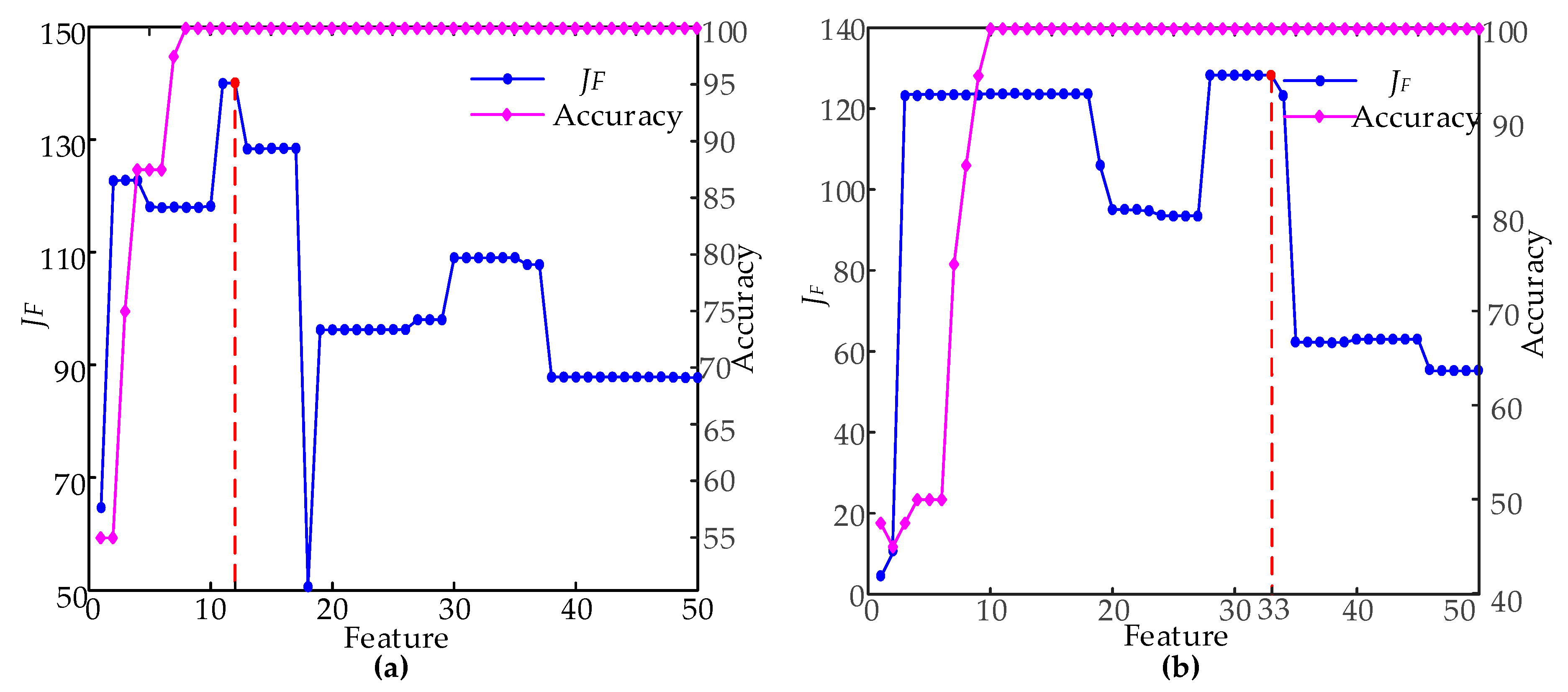
Figure 8 is the RF classification accuracy, and
JF is the feature selection process.
As it can be seen from
Figure 8, the accuracy of the feature subset dimension of the two segmentation scales was 100% when the feature subset dimensions were nine- and 10-dimensional, which cannot measure the effect from a single accuracy. With the increase in features, the evaluation index
JF of the feature subset first increased and then decreased. Finally, the maximum
JF value was used to determine the final feature subset. The best feature subset dimension were 12 and 33, when time domain segmentation scales were 29 and nine segments, respectively. At this time, when the time domain was divided into 29 segments and nine segments in the time domain,
JF reached the maximum value. When classifying with this feature subset, the class separability was the highest. Therefore,
JF and the feature dimension were considered comprehensively, and a classifier model was constructed, based on the best feature subset, with 12 dimensions of 29 segments. The best subsets of the features are shown in
Table 4.
6. Analysis of the Recognition Effect of the Hybrid Classifier with Unknown Faults
After determining the optimal subset of features, this paper designed an identification experiment with an unknown fault type, and verified the advantages of the hybrid classifier adopted by the new method. The screw loosening condition in the experiment was regarded as an unknown fault of the untrained sample, and it only participates in the final test without participating in the training process of the classifier. In the experiment, the error limit
and RBF kernel width parameter were 0.82 and 17.68, respectively [
27].
In order to compare the classification effects of multiple classifiers, RF and SVM were used to analyze normal and three fault types (the iron core stagnation, the screw loosening condition, and the poor lubrication condition) with untrained samples. The classifier to build the best feature subset was determined by the new method. SVM parameter reference [
9] setting. Among them, the screw looseness was regarded as an unknown fault state without training samples, and it participated in two classifiers but it did not participate in training. Twenty groups of normal samples of two known fault states (without an unknown type of fault) were used to train the classifier. Ten groups of normal samples of three fault states (with an unknown type of fault) were used to test the classifier. The classification results are shown in
Table 5.
From the results of
Table 5, RF and SVM accurately identified the fault types of the HVCBs. Neither RF nor SVM could identify an unknown fault type accurately (C3), in the state recognition without training samples. RF identified one group of samples as normal, four groups of samples were identified as iron core stagnation, and the five groups are identified as having poor lubrication condition, while SVM identified 10 groups of samples as being normal. The reliability of SVM was low. Therefore, the RF classifier has advantages, and its classification is more reliable.
In order to prove that the new method of the hierarchical hybrid classifier is used to identify the unknown type without training samples, a comparative test was carried out between the new method and the OCSVM-RF method.
Table 6 is the result of two hybrid classifiers for OCSVM-RF (O-R) and the new method OCSVM-RF-OCSVM (O-R-O). In contrast, O-R could make up for the shortcoming that RF mistakenly identified an unknown condition as a normal condition, but the 10 untrained samples were wrongly identified as known fault types.
7. Conclusions
This paper proposes a novel mechanical fault feature selection and diagnosis approach for HVCBs, using features extracted without signal processing. The signal is not processed by digital signal processing methods, and it extracts features directly in the time domain. Feature selection is used to gain the best feature subsets for achieving high efficiencies and accuracies of fault recognition. The main contribution of the new approach is as follows:
- (1)
The features is extracted directly after the time domain segmentation of the original signal, with less time complexity.
- (2)
Feature selection is adopted to reduce the optimal feature subset dimension, the time consuming nature of feature extraction, and the complexity of the classifier model.
- (3)
The hierarchical hybrid classifier avoids the limitation of identifying the fault samples as the normal condition, and identifies the unknown fault types effectively. Compared with the traditional multiple classifiers, the condition recognition effect is improved.
HVCB has many kinds of faults, degrees of faults. It is difficult to obtain all the data that is needed for relevant experiments. More samples of fault types and degree data for further experimental study will be accumulated in future work.


