Interactive OCT-Based Tooth Scan and Reconstruction

 , , , and
Abstract
1. Introduction
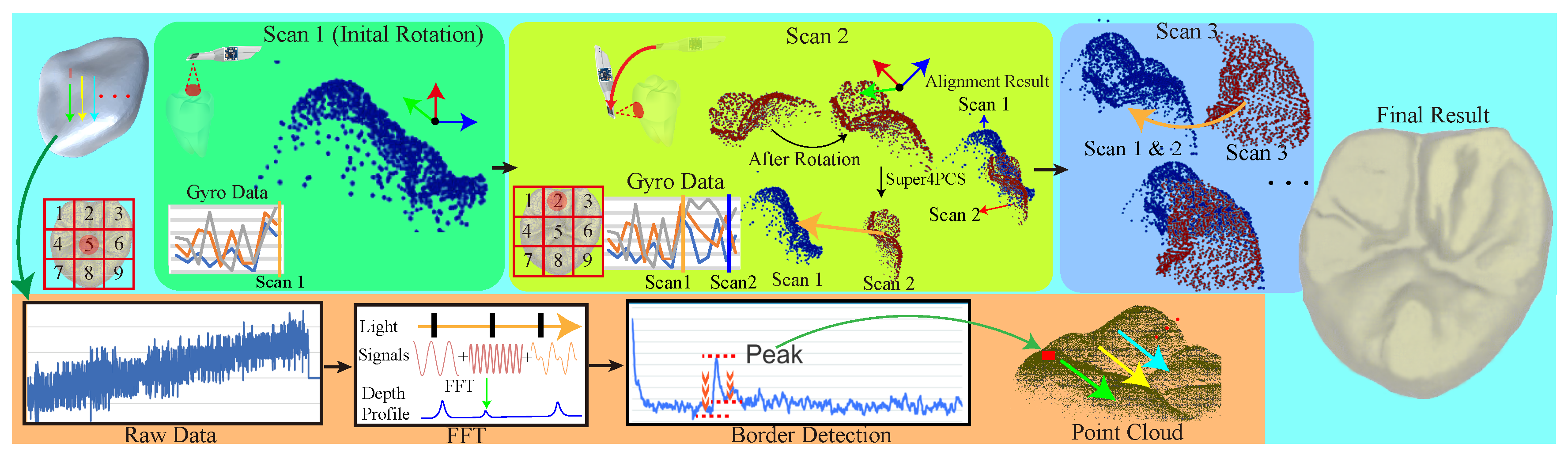
2. Overview
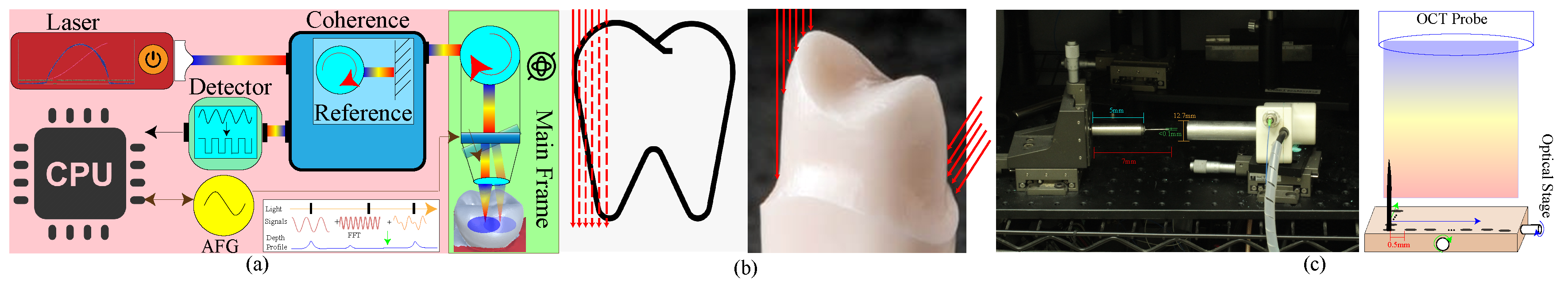
3. Swept-Source Optical Coherent Tomography
3.1. Injection and Reception Calibration
3.2. Three-Axis Posture Tracking Gyro
4. Interactive Dental Scanning
4.1. Boundary Detection
4.2. Parallelize Point-Cloud Alignment
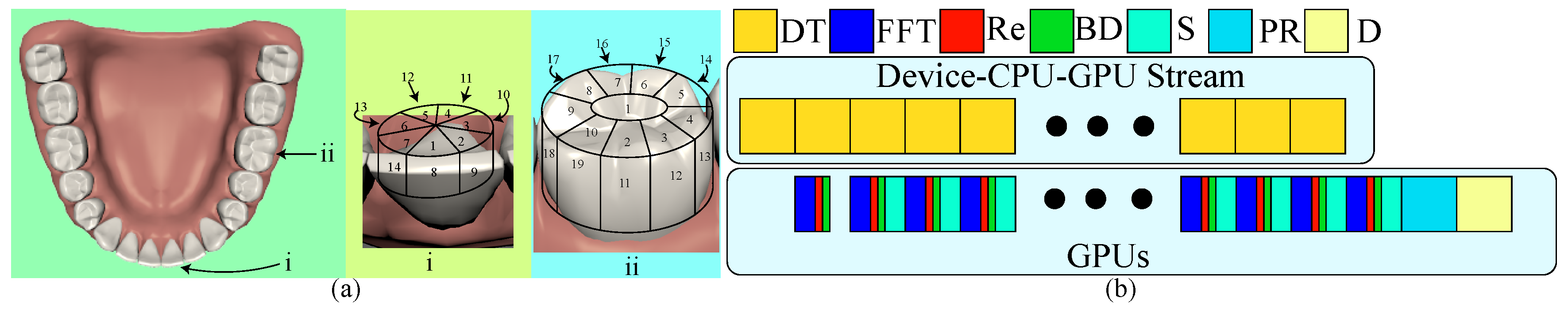
4.3. Effective Scanning Order
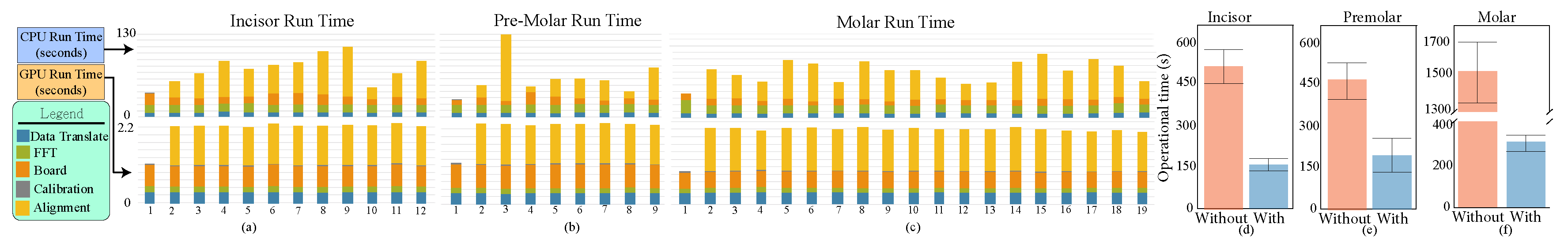
4.4. Streamlined Data Transfer and Computation
5. Surface Reconstruction
6. Results
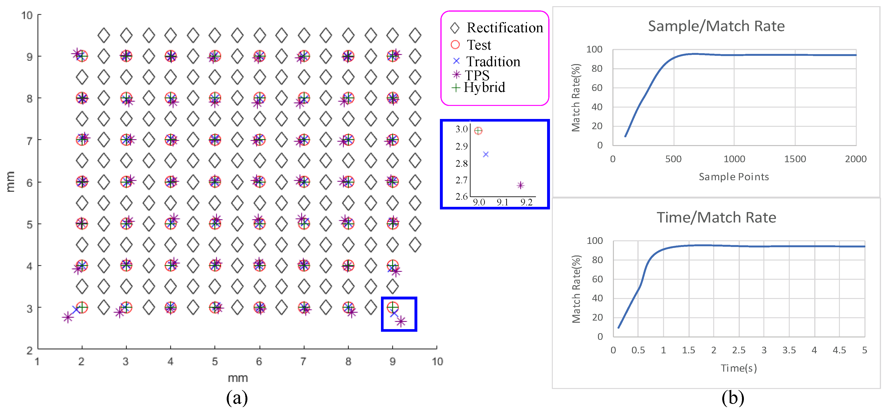
6.1. Ablation Study
6.2. Reconstruction Precision and Efficiency
6.3. Robustness of Scanning Ordering and Gyros
6.4. Usability Study
7. Conclusions
Author Contributions
Funding
Acknowledgments
Conflicts of Interest
Abbreviations
| OCT | Optical Coherence Tomography |
| GPU | Graphics Processing Unit |
| 4PCS | Super 4-Point-Congruent-Set |
| LIDAR | light detection and ranging |
| FFT | Fast Fourier Transform |
| CT | Computed Tomography |
| MRI | Magnetic Resonance Imaging |
| SSOCT | Swept-Source Optical Coherent Tomography |
| AFG | Arbitrary Function Generator |
| ADC | Analog-to-Digital Converter |
| TPS | Thin-Plate Spline |
| RANSAC | RANdom SAmple Consensus |
| DT | Transfer a slice of scanning data (DT) |
| Re | Optical Rectification (Re) |
| BD | Boundary Detection |
References
- Snavely, N.; Seitz, S.M.; Szeliski, R. Modeling the world from internet photo collections. Int. J. Comput. Vis. 2008, 80, 189–210. [Google Scholar] [CrossRef]
- Schönberger, J.L.; Radenović, F.; Chum, O.; Frahm, J. From single image query to detailed 3D reconstruction. In Proceedings of the 2015 IEEE Conference on Computer Vision and Pattern Recognition (CVPR), Boston, MA, USA, 7–12 June 2015; pp. 5126–5134. [Google Scholar]
- Autodesk Inc. Autodesk 123D apps. 2019. Available online: https://www.autodesk.com/solutions/123d-apps (accessed on 1 April 2019).
- Carestream Dental Inc. Carestream CS3600. 2019. Available online: https://www.carestreamdental.com/en-us/products/intraoral-scanners/cs-3600-dental/ (accessed on 1 April 2019).
- Izadi, S.; Kim, D.; Hilliges, O.; Molyneaux, D.; Newcombe, R.; Kohli, P.; Shotton, J.; Hodges, S.; Freeman, D.; Davison, A.; et al. KinectFusion: Real-time 3D Reconstruction and Interaction Using a Moving Depth Camera. In Proceedings of the 24th Annual ACM Symposium on User Interface Software and Technology (UIST ’11), Santa Barbara, CA, USA, 16–19 October 2011; pp. 559–568. [Google Scholar]
- Lai, K.; Bo, L.; Ren, X.; Fox, D. A large-scale hierarchical multi-view RGB-D object dataset. In Proceedings of the 2011 IEEE International Conference on Robotics and Automation, Shanghai, China, 9–13 May 2011; pp. 1817–1824. [Google Scholar]
- Li, Y.; Dai, A.; Guibas, L.; Nießner, M. Database-Assisted Object Retrieval for Real-Time 3D Reconstruction. Comput. Graph. Forum 2015, 34, 435–446. [Google Scholar] [CrossRef]
- Agatston, A.S.; Janowitz, W.R.; Hildner, F.J.; Zusmer, N.R.; Viamonte, M.; Detrano, R. Quantification of coronary artery calcium using ultrafast computed tomography. J. Am. Coll. Cardiol. 1990, 15, 827–832. [Google Scholar] [CrossRef]
- Ijiri, T.; Yoshizawa, S.; Yokota, H.; Igarashi, T. Flower Modeling via X-ray Computed Tomography. ACM Trans. Graph. 2014, 33, 48. [Google Scholar] [CrossRef]
- Ogawa, S.; Lee, T.M.; Kay, A.R.; Tank, D.W. Brain magnetic resonance imaging with contrast dependent on blood oxygenation. Proc. Natl. Acad. Sci. USA 1990, 87, 9868–9872. [Google Scholar] [CrossRef] [PubMed]
- Huang, D.; Swanson, E.A.; Lin, C.P.; Schuman, J.S.; Stinson, W.G.; Chang, W.; Hee, M.R.; Flotte, T.; Gregory, K. Optical Coherence Tomography. Science 1991, 254, 1178–1181. [Google Scholar] [CrossRef] [PubMed]
- Schmitt, J.M. Optical coherence tomography (OCT): A review. IEEE J. Sel. Top. Quantum Electron. 1999, 5, 1205–1215. [Google Scholar] [CrossRef]
- Colston, B.; Sathyam, U.; Dasilva, L.; Everett, M.; Stroeve, P.; Otis, L. Dental OCT. Opt. Express 1998, 3, 230–238. [Google Scholar] [CrossRef] [PubMed]
- Baumgartner, A.; Dichtl, S.; Hitzenberger, C.; Sattmann, H.; Robl, B.; Moritz, A.; Fercher, A.; Sperr, W. Polarization–sensitive optical coherence tomography of dental structures. Caries Res. 2000, 34, 59–69. [Google Scholar] [CrossRef] [PubMed]
- Colston, B.; Everett, M.; Silva, L.; Otis, L.; Nathel, H. Optical Coherence Tomography for Diagnosing Periodontal Disease. Proc. SPIE 1997, 2973, 216–220. [Google Scholar]
- Baek, J.H.; Na, J.; Lee, B.H.; Choi, E.; Son, W.S. Optical approach to the periodontal ligament under orthodontic tooth movement: A preliminary study with optical coherence tomography. Am. J. Orthod. Dentofac. Orthop. 2009, 135, 252–259. [Google Scholar] [CrossRef] [PubMed]
- Wilder-Smith, P.; Holtzman, J.; Epstein J, A. Optical diagnostics in the oral cavity: An overview. Oral Dis. 2010, 16, 717–728. [Google Scholar] [CrossRef] [PubMed]
- NVidia Inc. cuFFT. 2019. Available online: https://developer.nvidia.com/cufft (accessed on 1 April 2019).
- Mellado, N.; Aiger, D.; Mitra, N.J. Super 4pcs fast global pointcloud registration via smart indexing. Comput. Graph. Forum 2014, 33, 205–215. [Google Scholar] [CrossRef]
- Kazhdan, M.; Bolitho, M.; Hoppe, H. Poisson Surface Reconstruction. In Proceedings of the Fourth Eurographics Symposium on Geometry Processing (SGP ’06), Cagliari, Italy, 26–28 June 2006; pp. 61–70. [Google Scholar]
- Potsaid, B.; Baumann, B.; Huang, D.; Barry, S.; Cable, A.E.; Schuman, J.S.; Duker, J.S.; Fujimoto, J.G. Ultrahigh speed 1050 nm swept source/Fourier domain OCT retinal and anterior segment imaging at 100,000 to 400,000 axial scans per second. Opt. Express 2010, 18, 20029–20048. [Google Scholar] [CrossRef] [PubMed]
- Poddar, R.; Reddikumar, M. In vitro 3D anterior segment imaging in lamb eye with extended depth range swept source optical coherence tomography. Opt. Laser Technol. 2015, 67, 33–37. [Google Scholar] [CrossRef]
- Rother, C.; Kolmogorov, V.; Blake, A. Grabcut: Interactive foreground extraction using iterated graph cuts. ACM Trans. Graph. (TOG) 2004, 23, 309–314. [Google Scholar] [CrossRef]
- Kirk, R. Experimental Design: Procedures for the Behaviors Sciences, 2nd ed.; Brooks/Cole Publishing Company: Pacific Grove, CA, USA, 1982. [Google Scholar]


| Without (s) | With (s) | Acc. | |
|---|---|---|---|
| Incisor | 10.5 | ||
| %midrule Premolar | 14.8 | ||
| Molar | 14.8 |
© 2019 by the authors. Licensee MDPI, Basel, Switzerland. This article is an open access article distributed under the terms and conditions of the Creative Commons Attribution (CC BY) license (http://creativecommons.org/licenses/by/4.0/).
Share and Cite
Lai, Y.-C.; Lin, J.-Y.; Yao, C.-Y.; Lyu, D.-Y.; Lee, S.-Y.; Chen, K.-W.; Chen, I.-Y. Interactive OCT-Based Tooth Scan and Reconstruction. Sensors 2019, 19, 4234. https://doi.org/10.3390/s19194234
Lai Y-C, Lin J-Y, Yao C-Y, Lyu D-Y, Lee S-Y, Chen K-W, Chen I-Y. Interactive OCT-Based Tooth Scan and Reconstruction. Sensors. 2019; 19(19):4234. https://doi.org/10.3390/s19194234
Chicago/Turabian StyleLai, Yu-Chi, Jin-Yang Lin, Chih-Yuan Yao, Dong-Yuan Lyu, Shyh-Yuan Lee, Kuo-Wei Chen, and I-Yu Chen. 2019. "Interactive OCT-Based Tooth Scan and Reconstruction" Sensors 19, no. 19: 4234. https://doi.org/10.3390/s19194234
APA StyleLai, Y.-C., Lin, J.-Y., Yao, C.-Y., Lyu, D.-Y., Lee, S.-Y., Chen, K.-W., & Chen, I.-Y. (2019). Interactive OCT-Based Tooth Scan and Reconstruction. Sensors, 19(19), 4234. https://doi.org/10.3390/s19194234