1. Introduction
In industrial production, in order to ensure product quality or production safety, it is necessary to monitor the key process parameters or quality indicators in real time. However, online measurements are not always available, because the experimental analysis may be very time consuming, or analytical instruments may exceed acceptability. In these cases, soft sensors have been proposed and proved to be very practical, which are usually predictive models or systems built by using abundant data collected from industrial production. In recent years, soft sensors have become more and more popular in quality prediction and other applications related to process control [
1,
2].
According to a survey conducted by Japanese scholars, more than 90% of soft sensor models used in the Japanese chemical industry are based on linear modeling methods, including multiple linear regression (MLR), partial least squares (PLS), principal component analysis (PCA), and so on [
3]. In order to adapt to the nonlinearity of some industrial processes, several nonlinear modeling methods are also used, such as artificial neural network (ANN) [
4,
5], support vector machine (SVM), [
6,
7], nonlinear PLS [
8], and so on. Despite the above methods being popular, it is still not easy to continually keep the soft sensors in good performance. In order to build a good soft sensor, complex process changes have to be considered; otherwise, the accuracy of the soft sensor may decrease after a period of time. To cope with this problem, some adaptive methods, such as moving window techniques [
9] and recursive adaptation techniques [
10,
11], have been proposed. These methods can gradually adapt to new process states, but they cannot deal with abrupt changes such as catalyst failure and raw material changes [
12,
13].
In such situations, the just-in-time learning (JITL) method has been recently introduced to develop soft sensors, and it has successfully been used to control some industrial processes [
14,
15,
16,
17,
18]. In the JITL framework, there is no model that needs to be constructed offline in advance. When a prediction is required, the weight of each sample in the historical dataset is first calculated according to its similarity to the query sample; then, a local PLS model is constructed. After answering the query, the model is discarded. This means that every time a query arrives, the JITL-based method builds a new local model [
18]. Therefore, the JITL-based method can better cope with process changes, compared to global methods, and local model reconstruction also enables it to cope well with nonlinear processes [
17].
As one kind of JITL method, locally weighted PLS (LWPLS) can cope well with nonlinearity, collinearity, and process changes by combining the properties of PLS and locally weighted regression (LWR) [
19]. Therefore, it is very popular in various industrial applications. In LWPLS, several parts closely related to its performance need to be well selected, such as the bandwidth parameter, distance function, weight function, and so on. This paper focuses on the bandwidth parameter
h, which can be crucial to LWPLS, since it determines the range of the neighborhood and the shape of weight changes when a local PLS model needs to be constructed [
20,
21]. If the bandwidth
h is too small, the problem of overfitting will occur, and the reliability of the LWPLS model will also be affected. On the other hand, if it is too large, satisfactory accuracy will not be achieved [
21,
22]. Therefore, a scheme is required to decide the optimal bandwidth parameter.
Several typical methods have been used to determine this parameter. One method is to use a fixed bandwidth. Although this method is simple, it cannot achieve a satisfactory performance because the data density in the whole data set is likely to be very different. Another method is the k-nearest neighbor (K-NN) bandwidth method. In this method, the distance between the query point and each sample is first calculated and arranged in ascending order; then, the bandwidth is set to be the K-th distance value [
23]. Compared to the fixed bandwidth selection, the K-NN method performs better in various applications. However, it is not easy to determine an optimal K value for each query [
20,
21,
23]. The third method is the automatic bandwidth design method, in which the optimal bandwidth is determined by trial and error based on certain criteria, such as the minimum mean square error (MMSE) criterion or Akaike’s information criterion (AIC) [
22]. This method lacks the idea of optimization, and the accuracy needs to be further improved. In addition, some intelligent algorithms, such as the genetic algorithm (GA) [
21,
24] and particle swarm optimization (PSO) [
22], have been used to optimize the bandwidth. However, in these methods, bandwidth optimization, using the intelligent algorithm, is done online, which greatly affects the query response speed of the model.
To improve the model’s accuracy, while at the same time ensuring a rapid query response, a two-phase bandwidth optimization strategy, including a training phase and a prediction phase, is proposed by combining PSO and LWPLS. The proposed method is referred to as PSO-LWPLS, which integrates the basic idea of point-based local bandwidth selection [
20] and the K-NN method. Both offline and online operation schemes are designed to obtain the optimal bandwidth for each query. However, this is a single parameter optimization problem: why is PSO used instead of traditional one-dimensional search methods such as the Newton method, or the golden section search method (GSSM)? The objective of bandwidth optimization is to minimize the prediction error, so the relationship between the objective function and the bandwidth parameter is analyzed. The analysis results show that this relationship is complex and cannot be expressed by explicit mathematical formulas. In addition, when the density distribution of sample data is different, multiple minimum values could occur in the relationship curves between the objective function and the bandwidth value. The above two factors make the traditional one-dimensional search methods not applicable. This will be explained in detail in
Section 3.2.
The rest of this paper is arranged as follows.
Section 2 briefly describes the basic LWPLS and PSO algorithms. Then, in
Section 3, the proposed PSO-LWPLS modeling method is described in detail. Both numerical and industrial case studies are given in
Section 4. Finally, the paper is summarized in
Section 5.
3. The Proposed PSO–LWPLS Method
In this section, the bandwidth-tuning problem in LWPLS is first described. Then, why PSO was chosen is explained in detail. Finally, the proposed bandwidth optimization strategy is introduced.
3.1. Bandwidth Tuning Problem in LWPLS
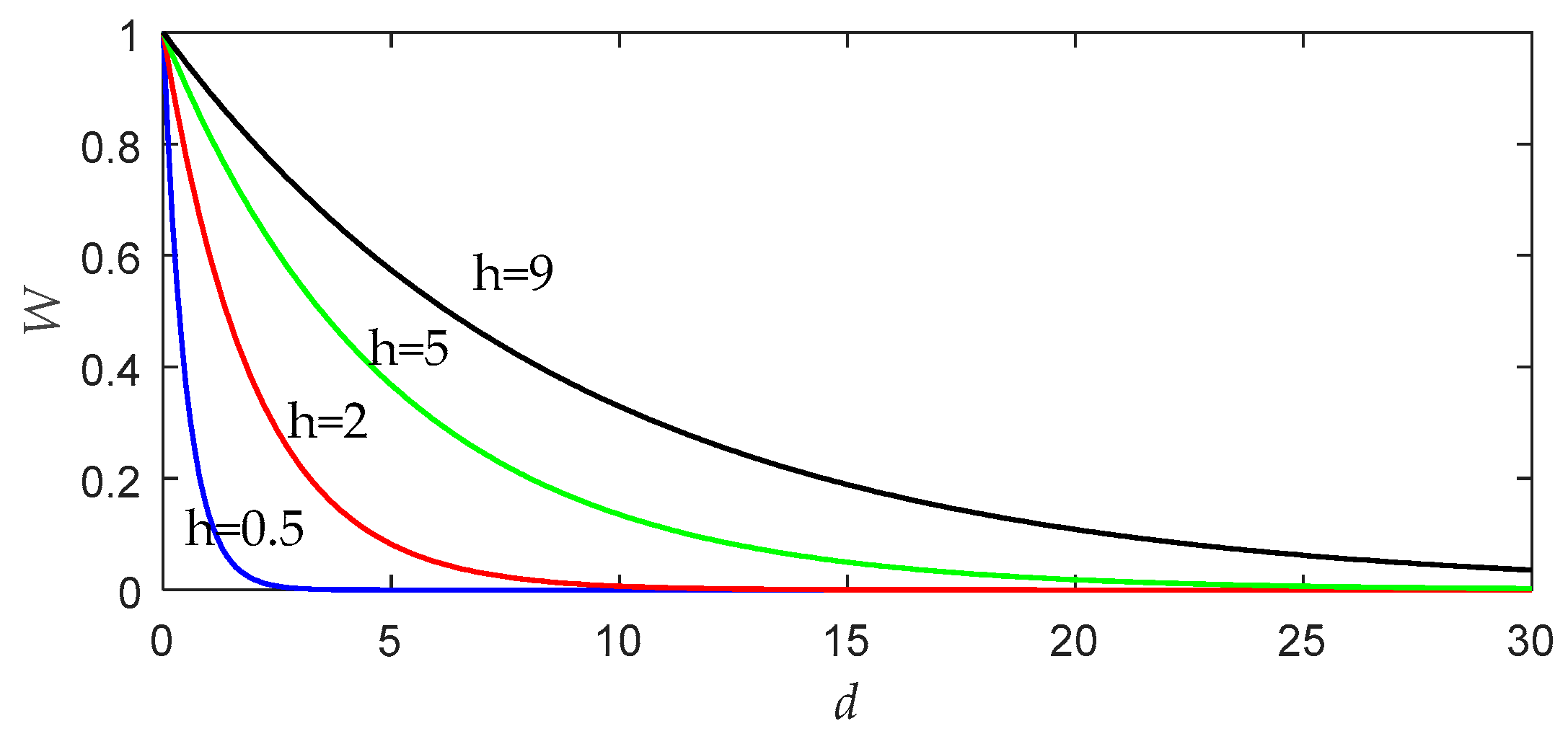
Similar to most learning algorithms, the LWPLS algorithm also requires parameter tuning to achieve a good performance. In LWPLS, the bandwidth is an important parameter that defines the range of the neighborhood, and the shape of the weight changes when a local PLS model is constructed [
20]. To illustrate the effect of bandwidth on the performance of LWPLS, we draw a graph, as shown in
Figure 1, according to the weight function defined by Equation (3).
As can be seen from
Figure 1, the bandwidth
h can control which samples play decisive roles in local modeling near the query point. If the bandwidth value increases, more remote samples will also have an opportunity to affect the query result. When
h tends to be infinite, the similarity of all data becomes equal to 1, and the LWPLS algorithm will be no different from the simple PLS algorithm. On the other hand, the smaller the bandwidth is, the faster the weight decreases. In this case, only a few samples close to the query point are used for local modeling. If
h is too small, the problem of overfitting will occur, and the reliability of the LWPLS model will also be affected [
21,
22].
Since the data density and distribution in the whole dataset are unlikely to be the same in different locations, it is necessary to design an optimal bandwidth for every query to ensure that every prediction can achieve satisfactory accuracy. In addition, online queries usually need to be answered in time, so computational overhead is also an important factor that cannot be ignored in bandwidth selection. Therefore, to improve the model’s accuracy without excessively increasing the computational overhead, a scheme is needed to determine the optimal bandwidth.
3.2. Why Use PSO?
To design an optimal bandwidth for each query is a single parameter optimization problem. Why is PSO used instead of one-dimensional search methods such as the golden section search method (GSSM) or the Newton method?
Based on the introduction of the LWPLS algorithm in
Section 2.1, one can see that the bandwidth parameter initially appears in the calculation of sample weight in Equation (3). The weights undergo complex transformations in the LWPLS operation process, and they have been applied a number of times to calculate intermediate variables, such as in constructing the matrix
and solving eigenvectors to obtain intermediate variables, solving latent variables and load vectors in LWPLS, and so on. Therefore, after these complex calculations and transformations, one cannot exactly know the relationship between the prediction error and the bandwidth parameter, and cannot express the relationship in an accurate mathematical expression.
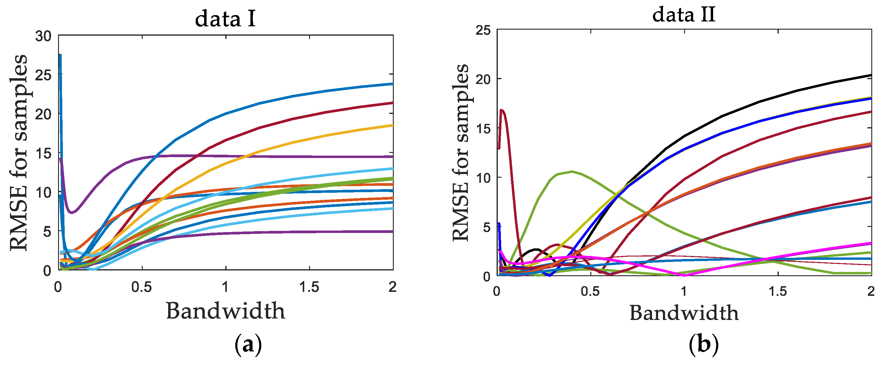
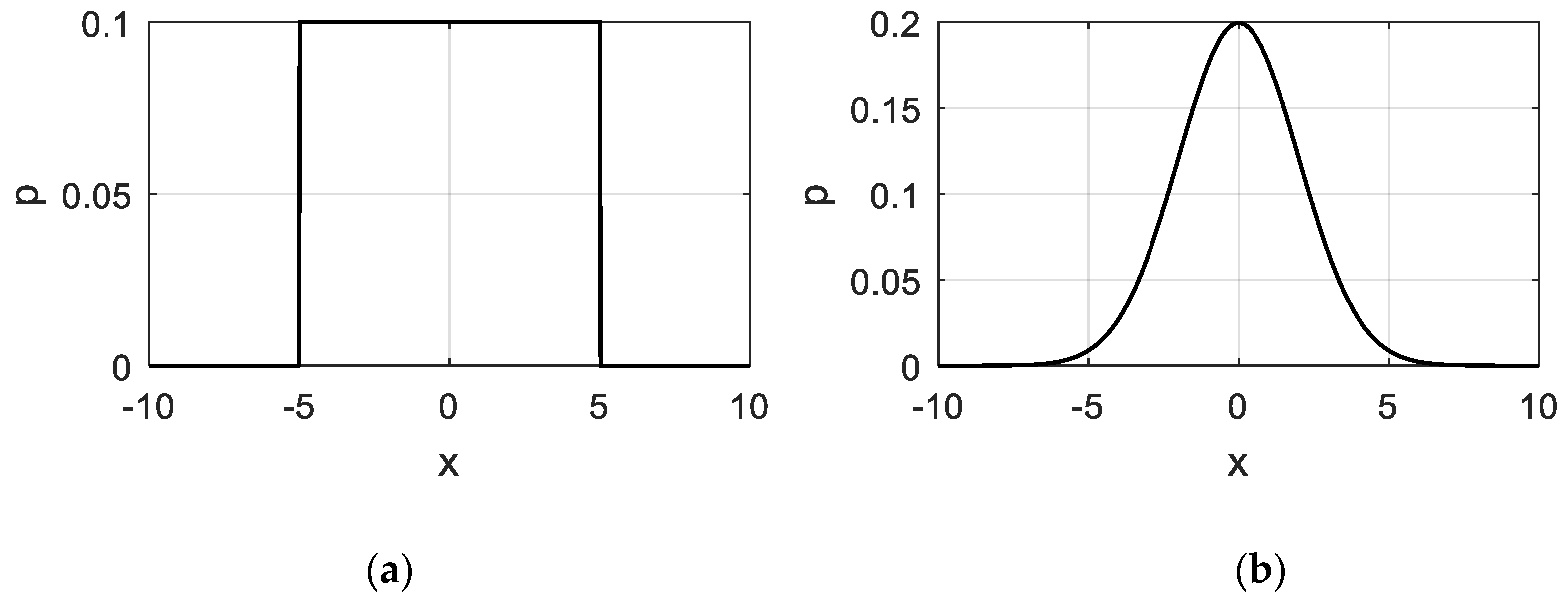
In addition, through numerical simulations, data set I with a uniform data density and data set II with a non-uniform data density are constructed. A series of bandwidth values are selected. For each data set, a number of sample points are randomly selected as test data. Each data set was tested independently, and the predicted values were obtained by using the LWPLS model. Then, for each test sample point, with each bandwidth value, repeated independent experiments were carried out, and the predicted root mean square error (RMSE) of the test sample was calculated. Then, the relationship curve of the RMSE with bandwidth values for each test sample was obtained, as shown in
Figure 2.
It can be seen for data set I that each RMSE curve basically had a unique minimum value that changed with the bandwidth, which corresponds to the optimal bandwidth of the sample, and the optimal bandwidth values of all test samples were very concentrated. For data set II, because of the uneven distribution of data, the optimal bandwidth values of different samples were relatively scattered, and some RMSE curves had multiple minimum values.
The above two factors can be summarized as follows: first, the relationship between the objective function and the bandwidth parameter is complex and cannot be expressed by explicit formulas; second, there may be multiple minimum values in the objective function. These two factors make some common one-dimensional search methods, such as the golden section search method (GSSM) and the Newton method, not applicable. However, as a kind of swarm intelligence algorithm, PSO itself has fewer requirements for the mathematical nature of the optimization problem. Therefore, in this paper, PSO is used in the bandwidth optimization problem. To verify its effectiveness, the PSO method was compared with the popular golden section search method in
Section 4.
3.3. Optimal Bandwidth Selection Using PSO
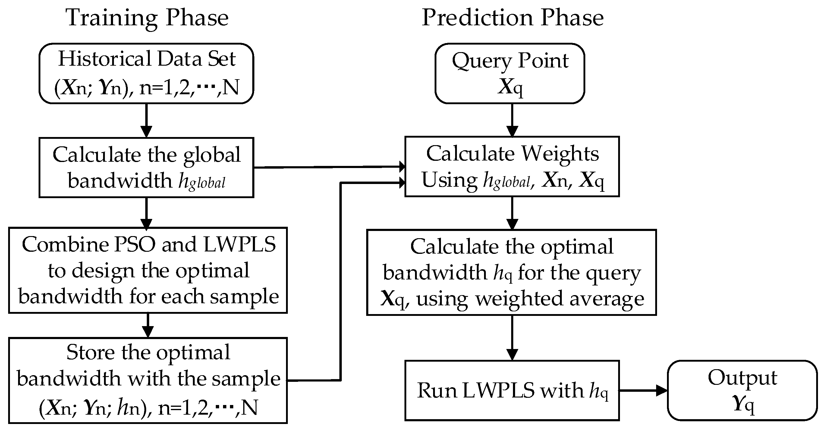
In this section, we introduce the hybrid PSO–LWPLS with a two-phase strategy to meet the above requirements, including a training phase and a prediction phase.
Figure 3 shows the framework of the proposed two-phase strategy. The idea of the point-based bandwidth selection and the K-NN method are combined together in this framework. The specific steps of the two phases are given below.
3.3.1. Training Phase
In the training phase, an optimal bandwidth is designed for each sample in the historical data set, so as to prepare the parameters for the prediction phase. PSO and LWPLS are both used to calculate the optimal bandwidth. Before calculation, the initial parameters of the PSO algorithm need to be set. In order to determine the bandwidth selection range (hmin, hmax), we first adopted the leave-one-out (LOO) cross-validation method to obtain the best global bandwidth hglobal. The global optimal bandwidth represents the average of the optimal bandwidth of all samples, and the optimal bandwidth of each sample basically fluctuates near the average. In practical applications, one can first give a test range based on the global bandwidth, such as hmin = 0.5 hglobal and hmax = 1.5 hglobal; then, the optimal bandwidth value of each training sample can be obtained by offline optimization calculations. If the optimal bandwidths of all samples are within this range, and the gap between the bandwidths and the range boundaries is not too large, it indicates that the above test range is reasonable. If the optimal bandwidths of some samples reach the boundary values, the range should be enlarged appropriately to ensure that each sample can search for the optimal bandwidth in the range. However, this range should not be too large to affect the convergence rate of PSO.
Although the whole training phase may seem time consuming, the computational cost is usually acceptable because all the calculations are done offline. The steps are as follows.
Step 1: Calculate the global optimal bandwidth hglobal using leave-one-out cross-validation.
Step 2: Combine PSO and LWPLS to design the optimal bandwidth for each sample, as described in the following procedure.
For one sample (
Xn;
Yn) of the historical data set, when calculating its corresponding bandwidth, it is used as a query, and the rest are taken as training samples. In this optimization problem, the particles represent various bandwidth values in the range (e.g.,
hmin = 0.5
hglobal,
hmax = 1.5
hglobal). The fitness function is defined as [
21]:
where
is the estimated output by the LWPLS algorithm. Aiming at maximizing the fitness function, the optimal bandwidth
hn corresponding to the sample (
Xn,
Yn) can be finally obtained by iterations of the PSO algorithm.
Step 3: Store the optimal bandwidth hn with the corresponding sample.
After completing the training phase, we can get a new data set with point-based optimal bandwidth, i.e., (Xn, Yn; hn), n = 1, 2, …, N.
3.3.2. Prediction Phase
The task of the prediction phase is to design an optimal bandwidth
hq for the given query
Xq and estimate the output
according to
hq. First, weights need to be calculated for every sample according to Equation (3). However, we note that before the optimal bandwidth
hq is obtained, the initial weight calculation itself requires a bandwidth h, which results in a Catch-22 situation [
31]. To solve this problem, the global bandwidth obtained during the training phase is used to calculate the initial sample weights, because the global bandwidth is obtained by sufficient cross-validation on the training sample set, which also makes full use of the information provided by the sample data. Besides, there is no more information to prove which initial value is optimal. If the initial bandwidth is set at random, greater risk and error may occur. The detailed calculation steps are as follows.
Step 1: Calculate the initial sample weights
based on global bandwidth:
where
represents the weight of the nth sample.
Step 2: Search through the entire training set for the K most similar samples and calculate
hq for the given query
Xq, using the weighted average as follows:
This is proposed according to reference [
20], (p. 15), Equation (5), called “Weighting the Data Directly”. It is based on the principle that a similar input produces a similar output. Based on this principle, one can infer that the optimal bandwidth of the query point should be close to the optimal bandwidth of the neighboring points in the sample set, since the data density distribution around the neighboring points should be similar. In the training phase, the optimal bandwidth of each sample has been obtained, so to calculate the optimal bandwidth of the query point, one can first determine K neighboring sample points around it, and then calculate the weighted average of their optimal bandwidths—that is, the optimal bandwidth of the query point. The weighted average method makes
hq less sensitive to the change of K value, and the optimal value of K (basically between 2–10) is easier to determine by the trial-and-error method. When K continues to increase, the optimal bandwidth is basically stable due to the attenuation of the weights in the above Equation (22).
Step 3: Run the LWPLS algorithm with query-based bandwidth hq to obtain the corresponding output estimation .


