GNSS/LiDAR-Based Navigation of an Aerial Robot in Sparse Forests

 and
and
Abstract
:1. Introduction
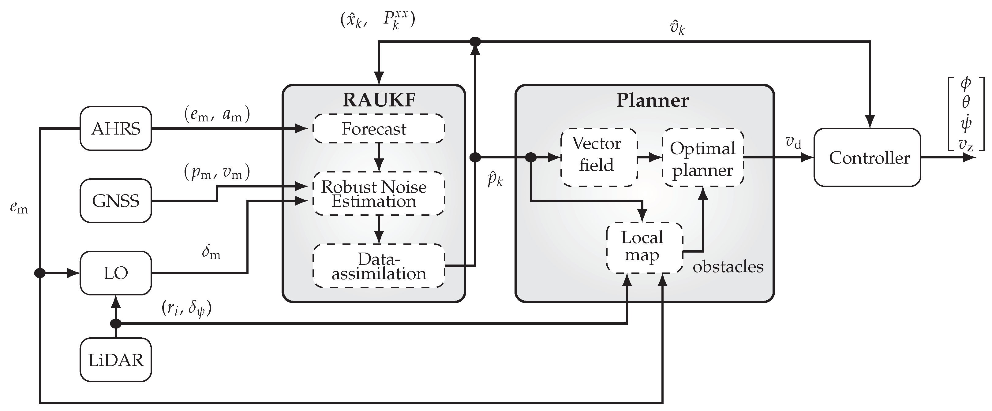
2. Problem Statement and Proposed Solution
3. Localization
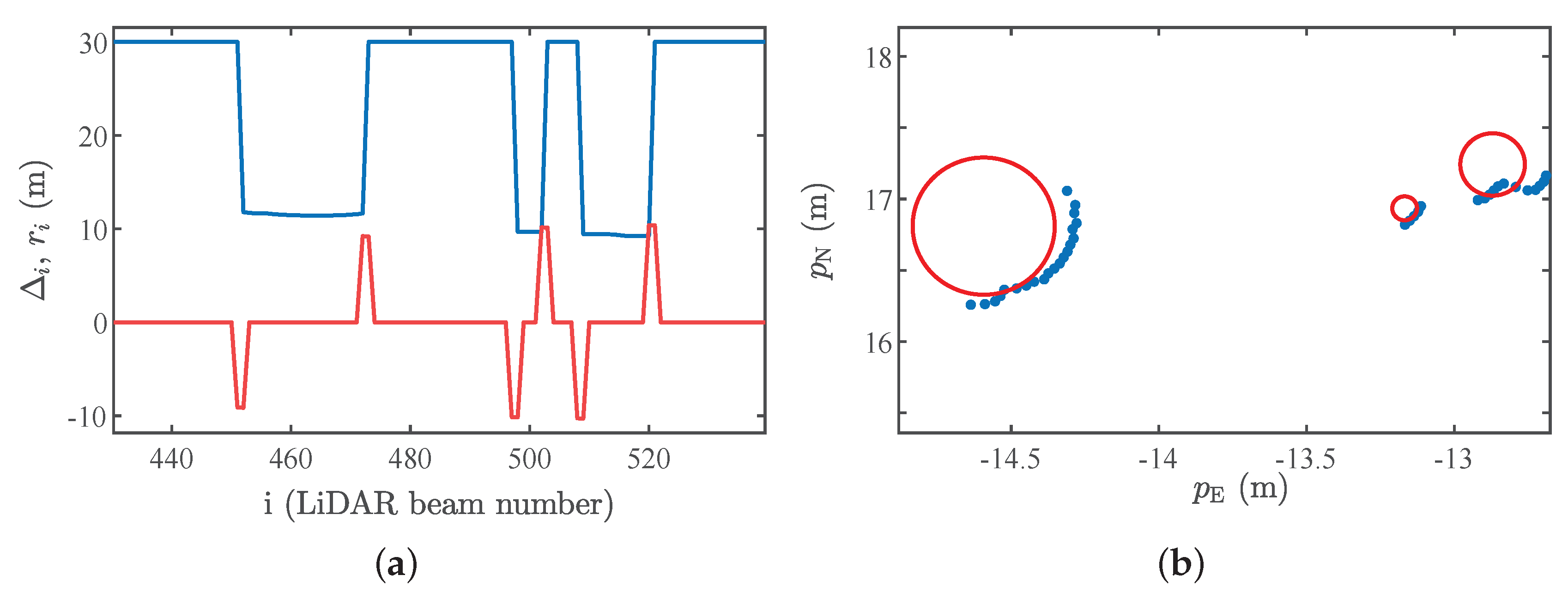
3.1. LiDAR-Based Motion Estimation in Forests
3.2. Mathematical Modeling
3.2.1. Process Model
3.2.2. Observation Model
3.3. Nonlinear State Estimator
3.3.1. Unscented Kalman Filter for Absolute and Relative Measurements
3.3.2. Adaptive Measurement Covariance Matrix
3.3.3. Outlier Rejection
3.3.4. Robust Adaptive Unscented Kalman Filter
4. Motion Control
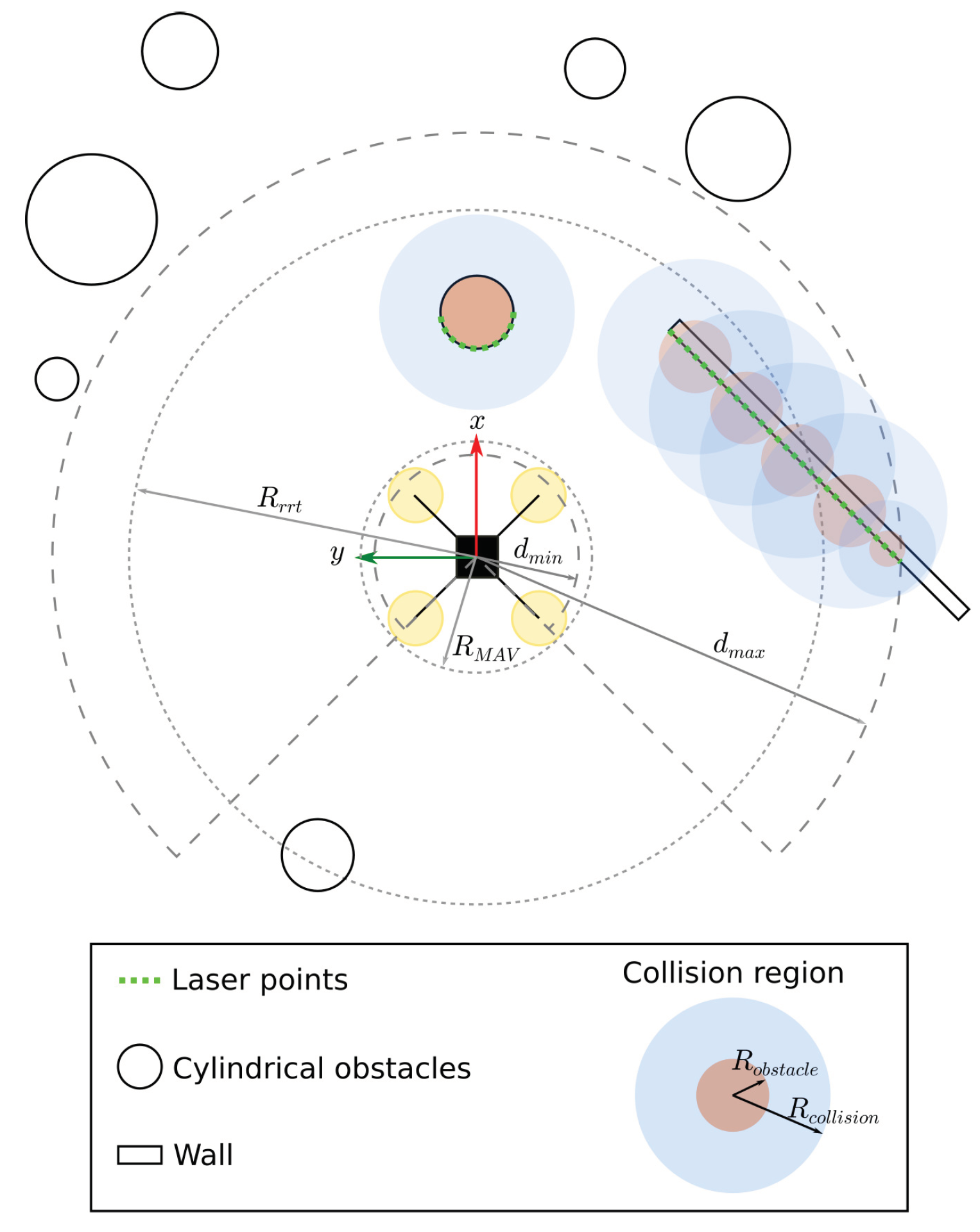
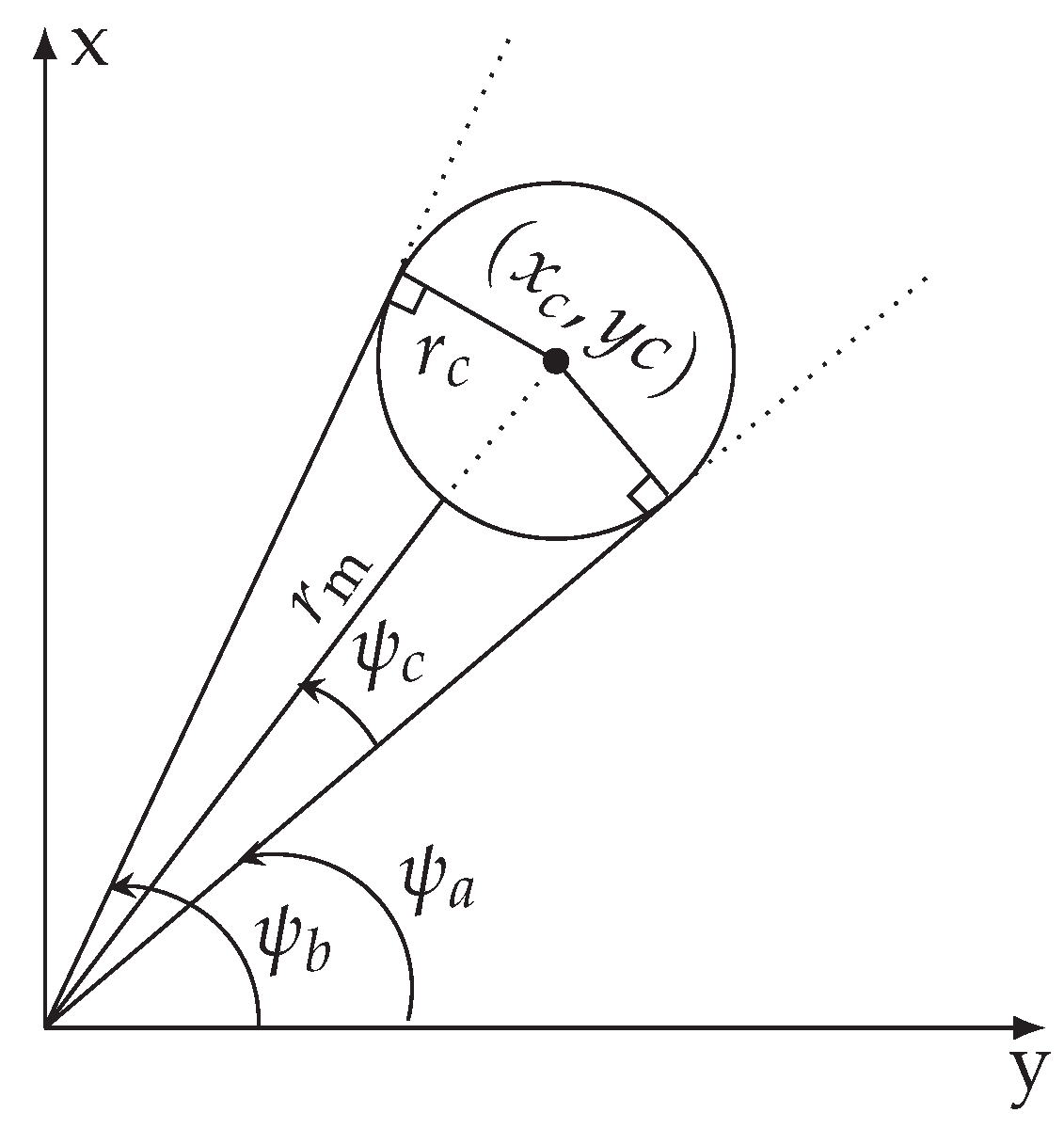
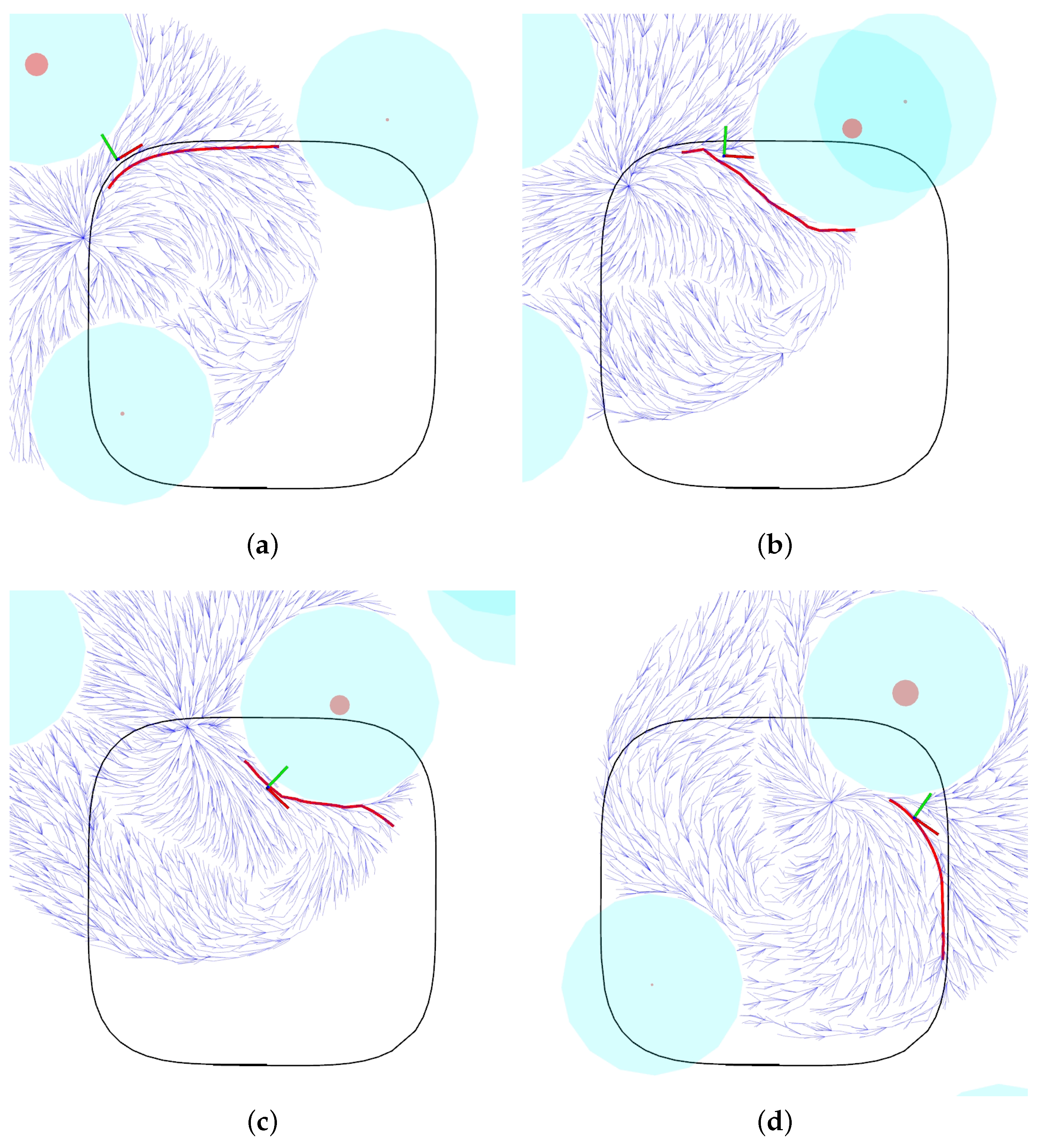
4.1. Local Mapping for Collision Avoidance
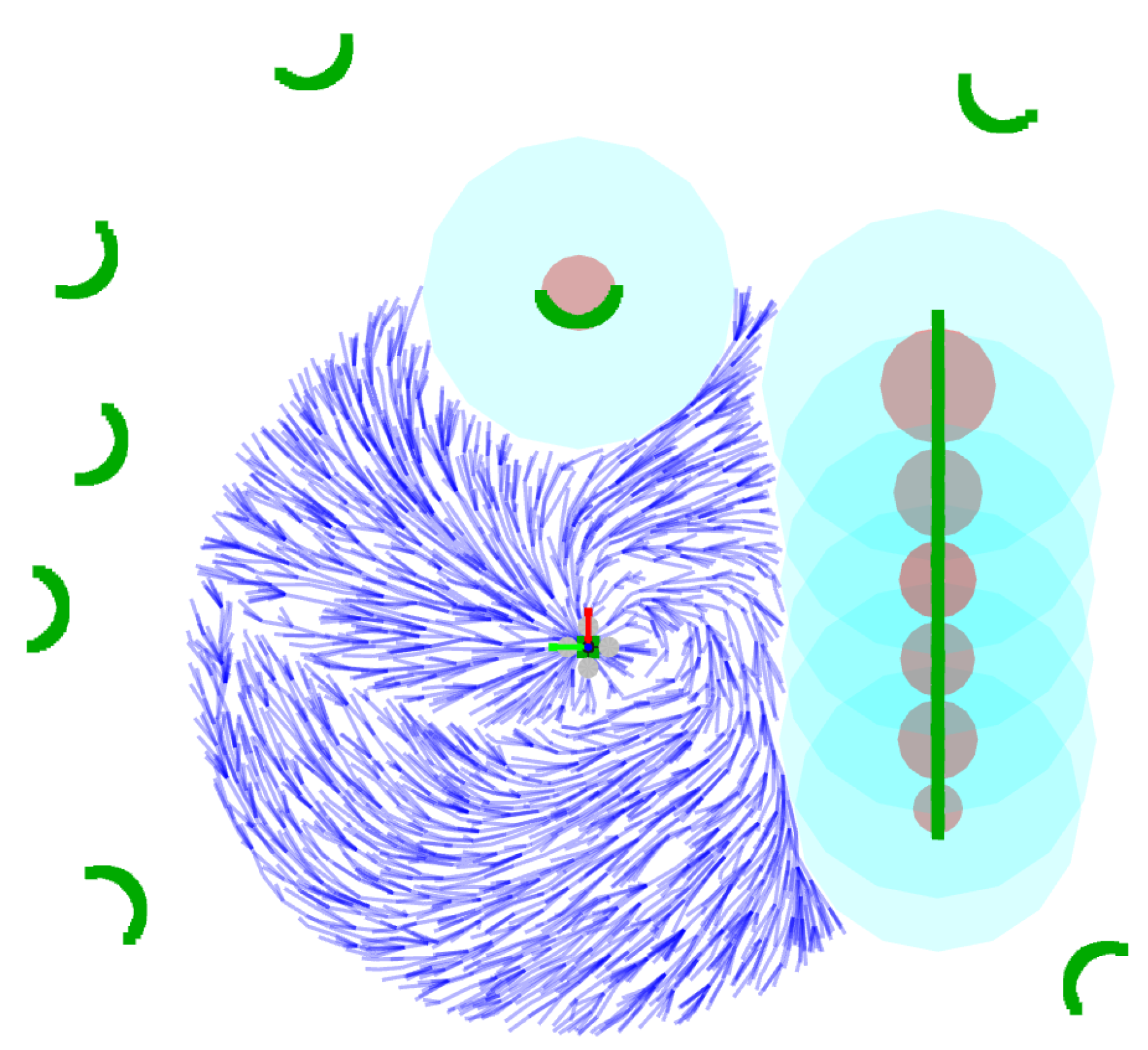
4.2. Path Planning
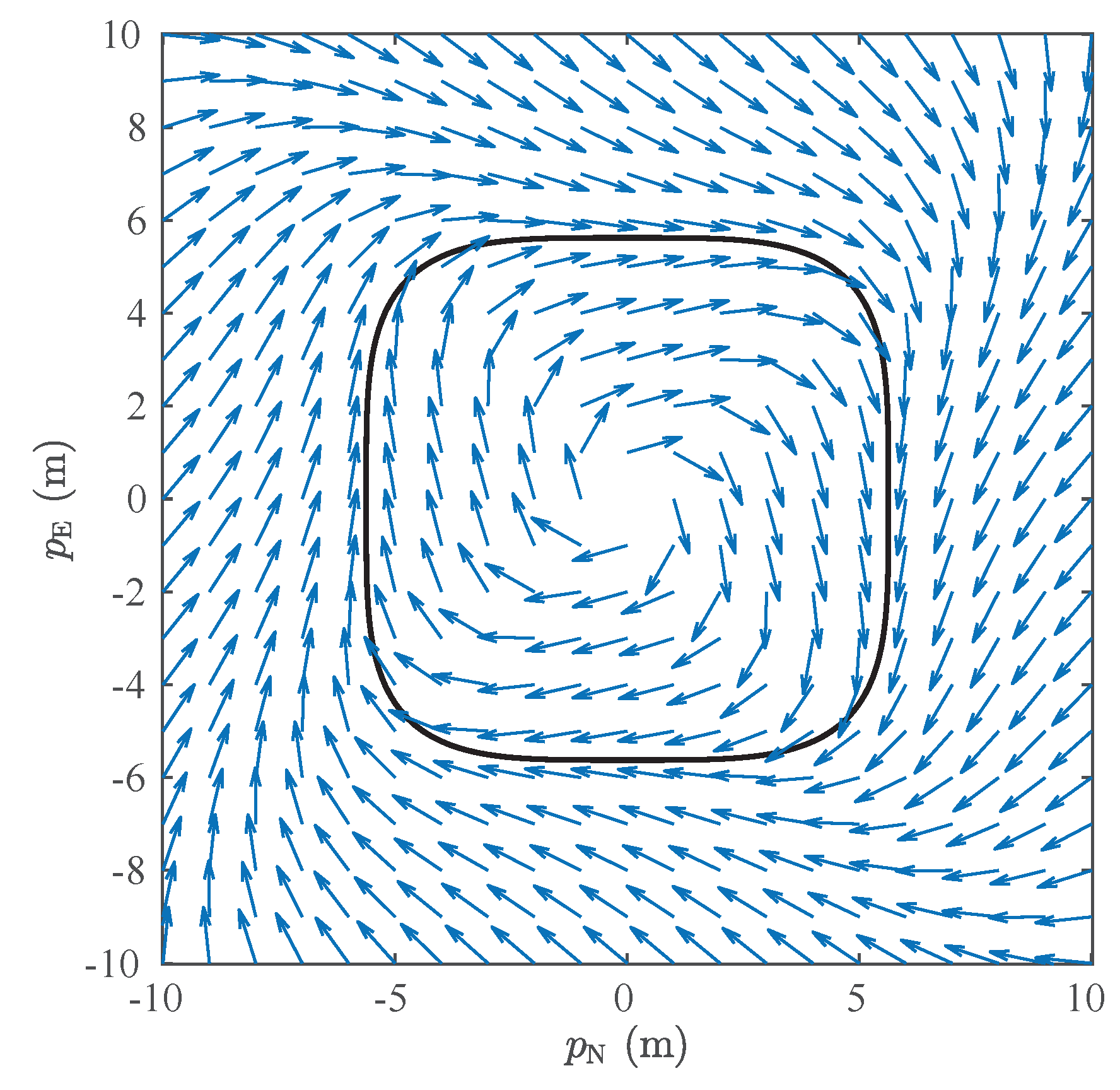
4.3. Path Following
5. Experimental Results
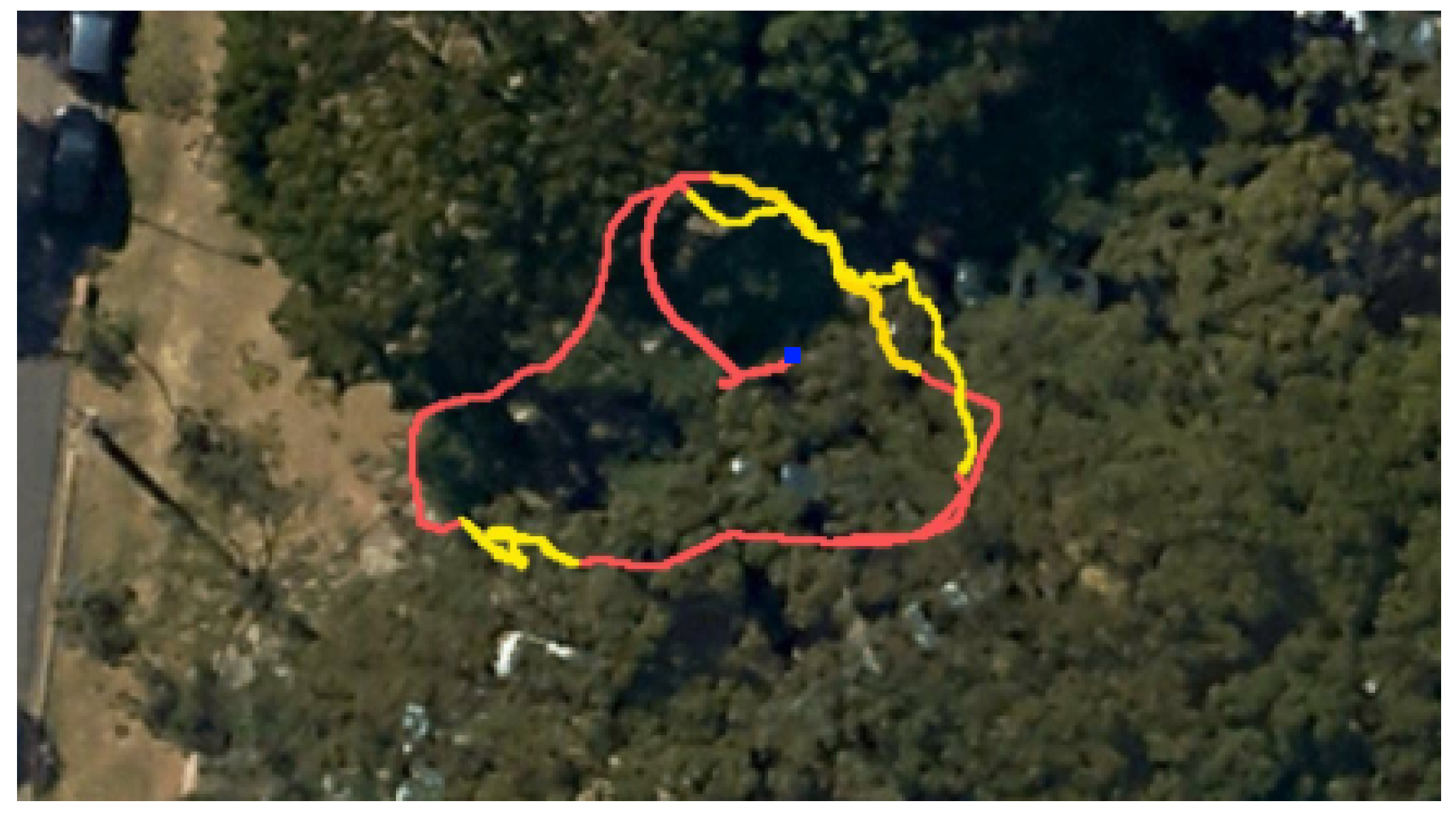
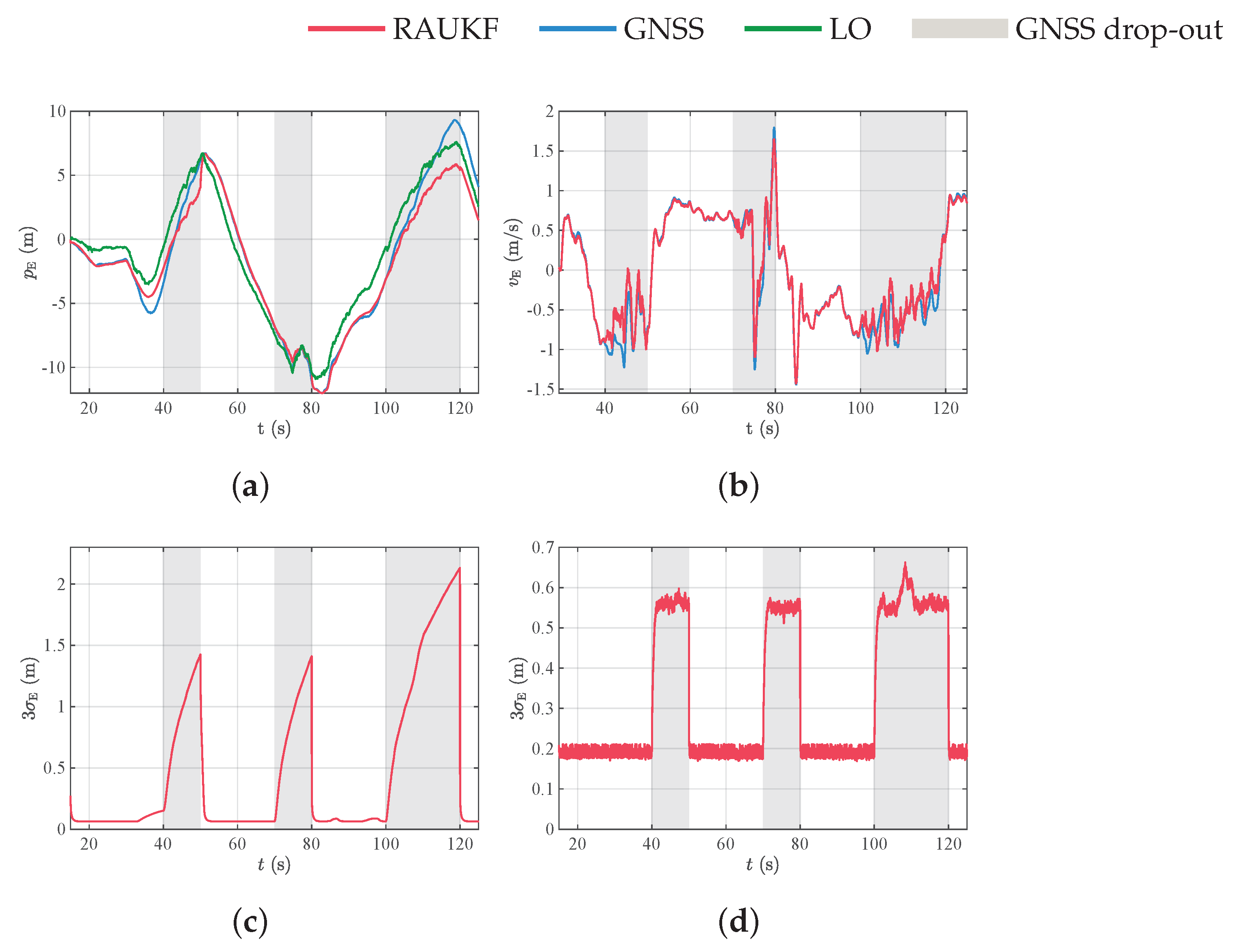
5.1. Localization System
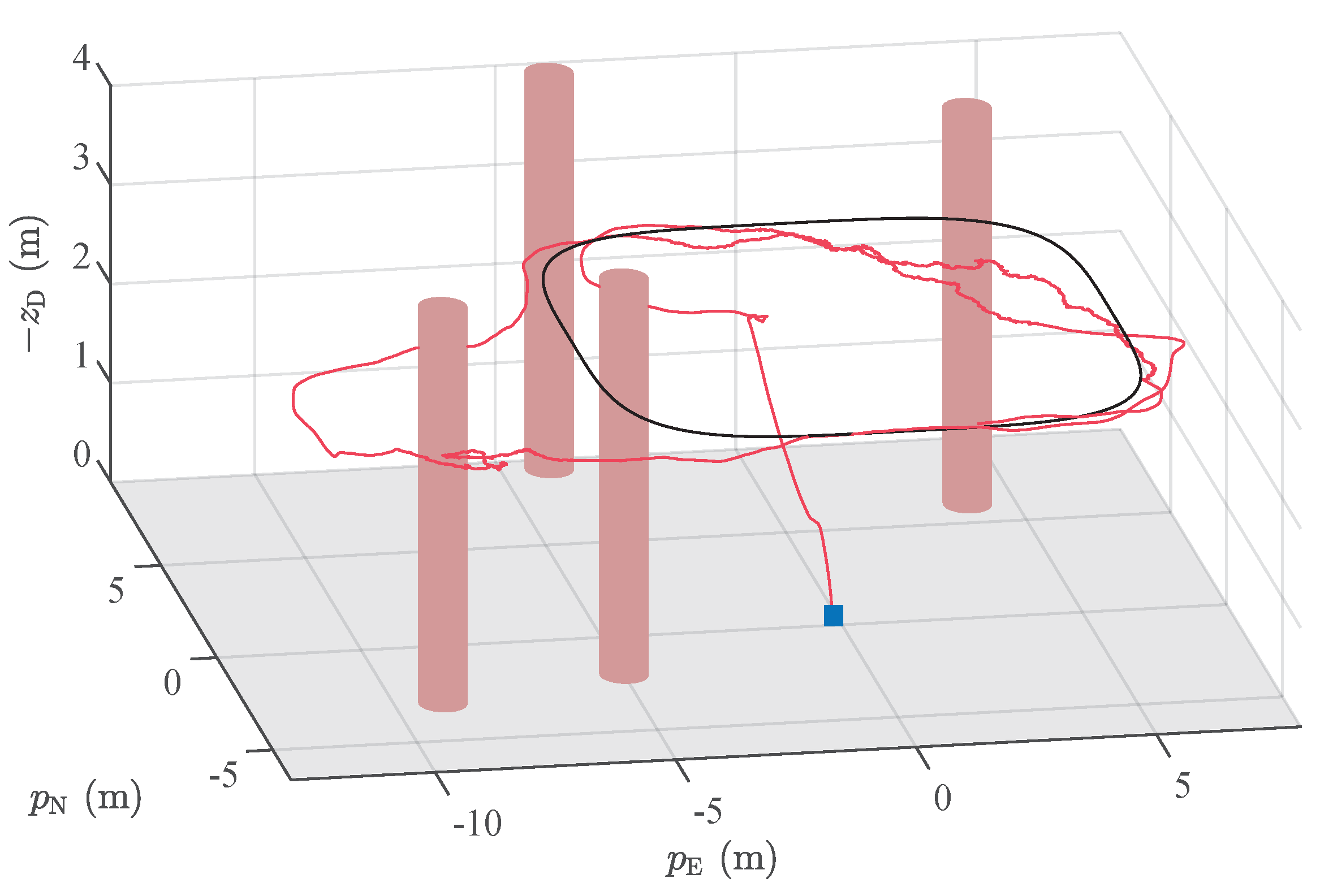
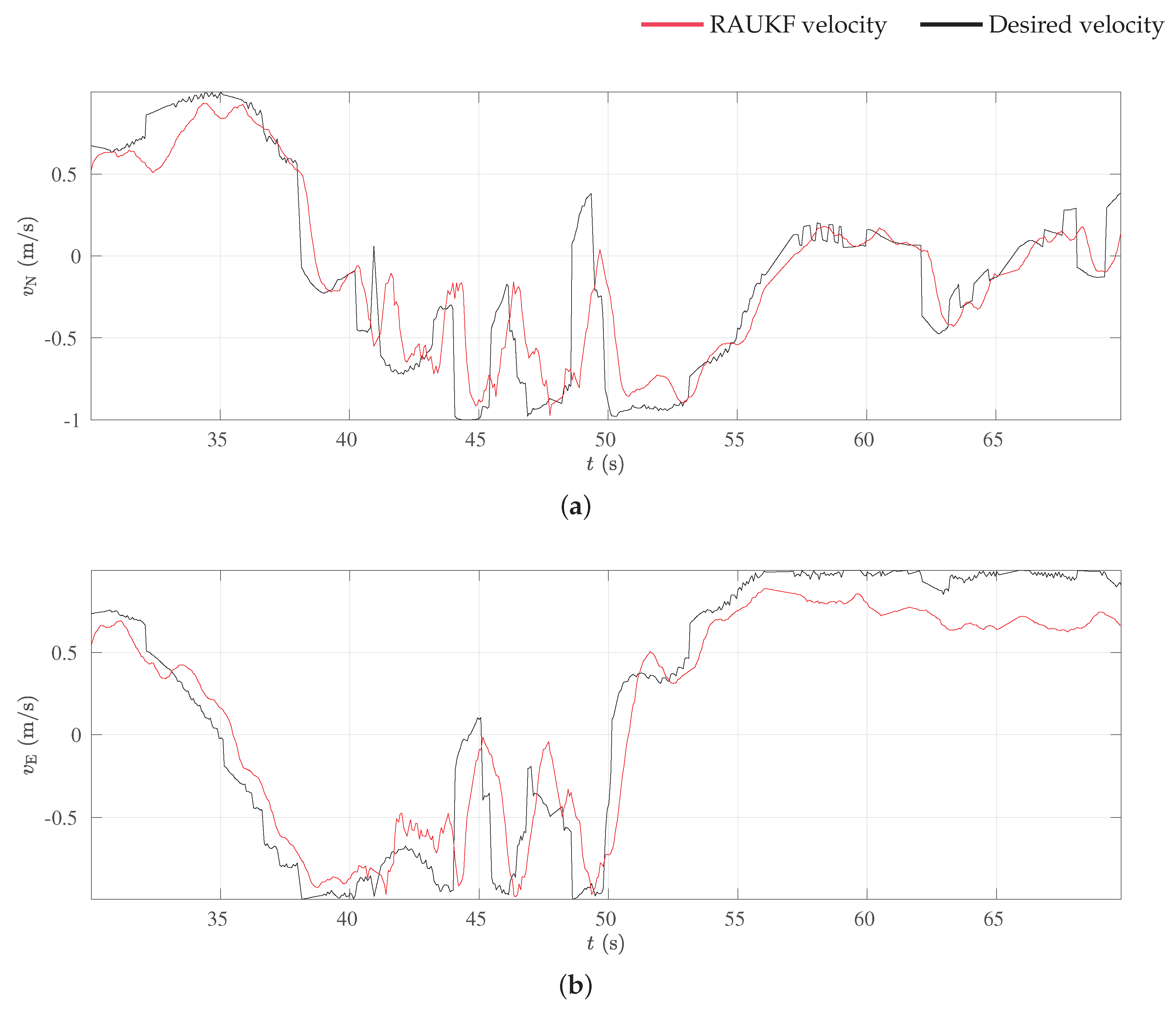
5.2. Motion Control System
6. Conclusions
Author Contributions
Funding
Acknowledgments
Conflicts of Interest
Notation
| position with respect to the NED coordinate frame. | |
| velocity with respect to NED coordinate frame. | |
| gravity acceleration vector, where m/s. | |
| rotation matrix between the body coordinate frame and the NED coordinate frame. | |
| input vector. | |
| accelerometer measurement. | |
| orientation measurement in unit quaternion. | |
| accelerometer bias. | |
| acceleration measurement noise. | |
| random walk noise. | |
| orientation measurement noise. | |
| cloned state vector. | |
| state vector. | |
| output measurement. | |
| position measurement given by GNSS. | |
| velocity measurement given by GNSS. | |
| position measurement noise. | |
| velocity measurement noise. | |
| relative measurement given by LO. | |
| relative measurement noise. | |
| process model. | |
| observation model. | |
| state estimate. | |
| covariance matrix of state estimate. | |
| process noise. | |
| covariance matrix of process noise. | |
| output measuremnt noise. | |
| covariance matrix of output measurement noise. | |
| nominal covariance matrix of output measurement noise. | |
| estimate of the covariance matrix of output measurement noise. | |
| innovation. | |
| normalized innovation squared. | |
| MAV’s path. | |
| vector field |
References
- Freitas, G.; Gleizer, G.; Lizarralde, F.; Hsu, L.; dos Reis, N.R.S. Kinematic reconfigurability control for an environmental mobile robot operating in the Amazon rain forest. J. Field Robot. 2010, 27, 197–216. [Google Scholar] [CrossRef]
- Morita, M.; Nishida, T.; Arita, Y.; Shige-eda, M.; di Maria, E.; Gallone, R.; Giannoccaro, N.I. Development of robot for 3D measurement of forest environment. J. Robot. Mech. 2018, 30, 145–154. [Google Scholar] [CrossRef]
- Belbachir, A.; Escareno, J.; Rubio, E.; Sossa, H. Preliminary results on UAV-based forest fire localization based on decisional navigation. In Proceedings of the 2015 Workshop on Research, Education and Development of Unmanned Aerial Systems (RED-UAS), Cancún, México, 23–25 November 2015; pp. 377–382. [Google Scholar]
- Karma, S.; Zorba, E.; Pallis, G.; Statheropoulos, G.; Balta, I.; Mikedi, K.; Vamvakari, J.; Pappa, A.; Chalaris, M.; Xanthopoulos, G.; et al. Use of unmanned vehicles in search and rescue operations in forest fires: Advantages and limitations observed in a field trial. Int. J. Disaster Risk Reduct. 2015, 13, 307–312. [Google Scholar] [CrossRef]
- Arroyo-Mora, J.P.; Kalacska, M.; Inamdar, D.; Soffer, R.; Lucanus, O.; Gorman, J.; Naprstek, T.; Schaaf, E.S.; Ifimov, G.; Elmer, K.; et al. Implementation of a UAV-Hyperspectral Pushbroom Imager for Ecological Monitoring. Drones 2019, 3, 12. [Google Scholar] [CrossRef]
- Krisanski, S.; Del Perugia, B.; Taskhiri, M.S.; Turner, P. Below-canopy UAS photogrammetry for stem measurement in radiata pine plantation. In Proceedings of the Remote Sensing for Agriculture, Ecosystems, and Hydrology XX, Berlin, Germany, 10–13 September 2018; Volume 10783, p. 1078309. [Google Scholar]
- Cui, J.Q.; Lai, S.; Dong, X.; Liu, P.; Chen, B.M.; Lee, T.H. Autonomous navigation of UAV in forest. In Proceedings of the 2014 International Conference on Unmanned Aircraft Systems (ICUAS), Orlando, FL, USA, 27–30 May 2014; pp. 726–733. [Google Scholar]
- Shen, S.; Mulgaonkar, Y.; Michael, N.; Kumar, V. Multi-sensor fusion for robust autonomous flight in indoor and outdoor environments with a rotorcraft MAV. In Proceedings of the 2014 IEEE International Conference on Robotics and Automation (ICRA), Hong Kong, China, 31 May–5 June 2014; pp. 4974–4981. [Google Scholar]
- Chambers, A.; Scherer, S.; Yoder, L.; Jain, S.; Nuske, S.; Singh, S. Robust multi-sensor fusion for micro aerial vehicle navigation in GPS-degraded/denied environments. In Proceedings of the 2014 American Control Conference, Portland, OR, USA, 4–6 June 2014; pp. 1892–1899. [Google Scholar]
- Strelow, D.; Singh, S. Motion estimation from image and inertial measurements. Int. J. Robot. Res. 2004, 23, 1157–1195. [Google Scholar] [CrossRef]
- Weiss, S.; Achtelik, M.W.; Lynen, S.; Achtelik, M.C.; Kneip, L.; Chli, M.; Siegwart, R. Monocular Vision for Long-term Micro Aerial Vehicle State Estimation: A Compendium. J. Field Robot. 2013, 30, 803–831. [Google Scholar] [CrossRef]
- Shen, S.; Michael, N.; Kumar, V. Autonomous multi-floor indoor navigation with a computationally constrained MAV. In Proceedings of the 2011 IEEE International Conference on Robotics and Automation, Shanghai, China, 9–13 May 2011; pp. 20–25. [Google Scholar]
- Tang, J.; Chen, Y.; Niu, X.; Wang, L.; Chen, L.; Liu, J.; Shi, C.; Hyyppä, J. LiDAR scan matching aided inertial navigation system in GNSS-denied environments. Sensors 2015, 15, 16710–16728. [Google Scholar] [CrossRef] [PubMed]
- Roumeliotis, S.I.; Burdick, J.W. Stochastic cloning: A generalized framework for processing relative state measurements. In Proceedings of the 2002 IEEE International Conference on Robotics and Automation (Cat. No. 02CH37292), Washington, DC, USA, 11–15 May 2002; Volume 2, pp. 1788–1795. [Google Scholar]
- Song, Y.; Nuske, S.; Scherer, S. A Multi-Sensor Fusion MAV State Estimation from Long-Range Stereo, IMU, GPS and Barometric Sensors. Sensors 2017, 17, 11. [Google Scholar] [CrossRef] [PubMed]
- Mehra, R. Approaches to adaptive filtering. IEEE Trans. Autom. Control 1972, 17, 693–698. [Google Scholar] [CrossRef]
- Li, X.R.; Bar-Shalom, Y. A recursive multiple model approach to noise identification. IEEE Trans. Aerosp. Electron. Syst. 1994, 30, 671–684. [Google Scholar] [CrossRef]
- Hide, C.; Moore, T.; Smith, M. Adaptive Kalman filtering algorithms for integrating GPS and low cost INS. In Proceedings of the Position Location and Navigation Symposium, Monterey, CA, USA, 26–29 April 2004; pp. 227–233. [Google Scholar]
- Chiella, A.C.B.; Teixeira, B.O.S.; Pereira, G.A.S. Robust attitude estimation using an adaptive unscented Kalman filter (forthcoming). In Proceedings of the 2019 IEEE International Conference on Robotics and Automation (ICRA), Montreal, QC, Canada, 20–24 May 2019. [Google Scholar]
- Cui, J.; Wang, F.; Dong, X.; Yao, K.A.Z.; Chen, B.M.; Lee, T.H. Landmark extraction and state estimation for UAV operation in forest. In Proceedings of the 32nd Chinese Control Conference, Xi’an, China, 26–28 July 2013; pp. 5210–5215. [Google Scholar]
- Chiella, A.C.B.; Teixeira, B.O.S.; Pereira, G.A.S. Quaternion-Based Robust Attitude Estimation Using an Adaptive Unscented Kalman Filter. Sensors 2019, 19, 2372. [Google Scholar] [CrossRef] [PubMed]
- Chiella, A.C.; Teixeira, B.O.S.; Pereira, G.A.S. State Estimation for Aerial Vehicles in Forest Environments. In Proceedings of the International Conference on Unmanned Aircraft Systems (ICUAS’19), Atlanta, GA, USA, 11–14 June 2019; pp. 882–890. [Google Scholar]
- Pereira, G.A.S.; Choudhury, S.; Scherer, S. A framework for optimal repairing of vector field-based motion plans. In Proceedings of the 2016 International Conference on Unmanned Aircraft Systems (ICUAS), Arlington, VA, USA, 7–10 June 2016; pp. 261–266. [Google Scholar]
- Gonçalves, V.M.; Pimenta, L.C.A.; Maia, C.A.; Dutra, B.C.O.; Pereira, G.A.S. Vector Fields for Robot Navigation Along Time-Varying Curv es in n-dimensions. IEEE Trans. Robot. 2010, 26, 647–659. [Google Scholar] [CrossRef]
- Karaman, S.; Frazzoli, E. Sampling-based algorithms for optimal motion planning. Int. J. Robot. Res. 2011, 30, 846–894. [Google Scholar] [CrossRef]
- Jutila, J.; Kannas, K.; Visala, A. Tree Measurement in Forest by 2D Laser Scanning. In Proceedings of the 2007 International Symposium on Computational Intelligence in Robotics and Automation, Jacksonville, FI, USA, 20–23 June 2007; pp. 491–496. [Google Scholar]
- Rusinkiewicz, S.; Levoy, M. Efficient variants of the ICP algorithm. In Proceedings of the Third International Conference on 3-D Digital Imaging and Modeling, Quebec City, QC, Canada, 28 May–1 June 2001; pp. 145–152. [Google Scholar]
- Lourenço, P.; Guerreiro, B.J.; Batista, P.; Oliveira, P.; Silvestre, C. Uncertainty characterization of the orthogonal procrustes problem with arbitrary covariance matrices. Pattern Recognit. 2017, 61, 210–220. [Google Scholar] [CrossRef]
- Beard, R.W.; McLain, T.W. Small Unmanned Aircraft: Theory and Practice; Princeton University Press: Princeton, NJ, USA, 2012. [Google Scholar]
- Simon, D. Optimal State Estimation: Kalman, H Infinity, and Nonlinear Approaches; John Wiley & Sons: Hoboken, NJ, USA, 2006. [Google Scholar]
- Julier, S.J.; Uhlmann, J.K. Unscented filtering and nonlinear estimation. Proc. IEEE 2004, 92, 401–422. [Google Scholar] [CrossRef]
- Xiong, K.; Zhang, H.; Chan, C. Performance evaluation of UKF-based nonlinear filtering. Automatica 2006, 42, 261–270. [Google Scholar] [CrossRef]
- ZhiWen, X.; XiaoPing, H.; JunXiang, L. Robust innovation-based adaptive Kalman filter for INS/GPS land navigation. In Proceedings of the Chinese Automation Congress (CAC), Changsha, China, 7–8 November 2013; pp. 374–379. [Google Scholar]
- Bialkowski, J.; Karaman, S.; Frazzoli, E. Massively parallelizing the RRT and the RRT*. In Proceedings of the 2011 IEEE/RSJ International Conference on Intelligent Robots and Systems, Francisco, CA, USA, 25–30 September 2011; pp. 3513–3518. [Google Scholar]


| Component | Hardware |
|---|---|
| Quadrotor | DJI Matrice 100 with IMU, barometer, magnetometer and GNSS sensors |
| Flight controller | DJI N1 |
| ESC/motor | DJI E Series 620D / DJI 3510 |
| Onboard computer | Odroid XU4 with an octa-core ARM processor, 2 GB of RAM, |
| running Ubuntu Mate 16.04 | |
| LiDAR | Hokuyo UTM-30LX-EW, 40 Hz, 30 m, scanning range |
| Servo-motor | Dynamixel MX-106R |
| USB/RS485 adapter | USB2Dynamixel |
| USB/TTL adapter | D-SUN, USB to TTL, CP2102 |
© 2019 by the authors. Licensee MDPI, Basel, Switzerland. This article is an open access article distributed under the terms and conditions of the Creative Commons Attribution (CC BY) license (http://creativecommons.org/licenses/by/4.0/).
Share and Cite
Chiella, A.C.B.; Machado, H.N.; Teixeira, B.O.S.; Pereira, G.A.S. GNSS/LiDAR-Based Navigation of an Aerial Robot in Sparse Forests. Sensors 2019, 19, 4061. https://doi.org/10.3390/s19194061
Chiella ACB, Machado HN, Teixeira BOS, Pereira GAS. GNSS/LiDAR-Based Navigation of an Aerial Robot in Sparse Forests. Sensors. 2019; 19(19):4061. https://doi.org/10.3390/s19194061
Chicago/Turabian StyleChiella, Antonio C. B., Henrique N. Machado, Bruno O. S. Teixeira, and Guilherme A. S. Pereira. 2019. "GNSS/LiDAR-Based Navigation of an Aerial Robot in Sparse Forests" Sensors 19, no. 19: 4061. https://doi.org/10.3390/s19194061
APA StyleChiella, A. C. B., Machado, H. N., Teixeira, B. O. S., & Pereira, G. A. S. (2019). GNSS/LiDAR-Based Navigation of an Aerial Robot in Sparse Forests. Sensors, 19(19), 4061. https://doi.org/10.3390/s19194061