Deep Learning for Industrial Computer Vision Quality Control in the Printing Industry 4.0
Abstract
1. Introduction
2. Evolution towards Automatic Deep Learning-Based OQC
3. Deep Learning for Industrial Computer Vision Quality Control
3.1. Deep Neural Network Architecture for Computer Vision in Industrial Quality Control in the Printing Industry 4.0
3.1.1. Experimental Setup
3.1.2. Data Pre-Processing
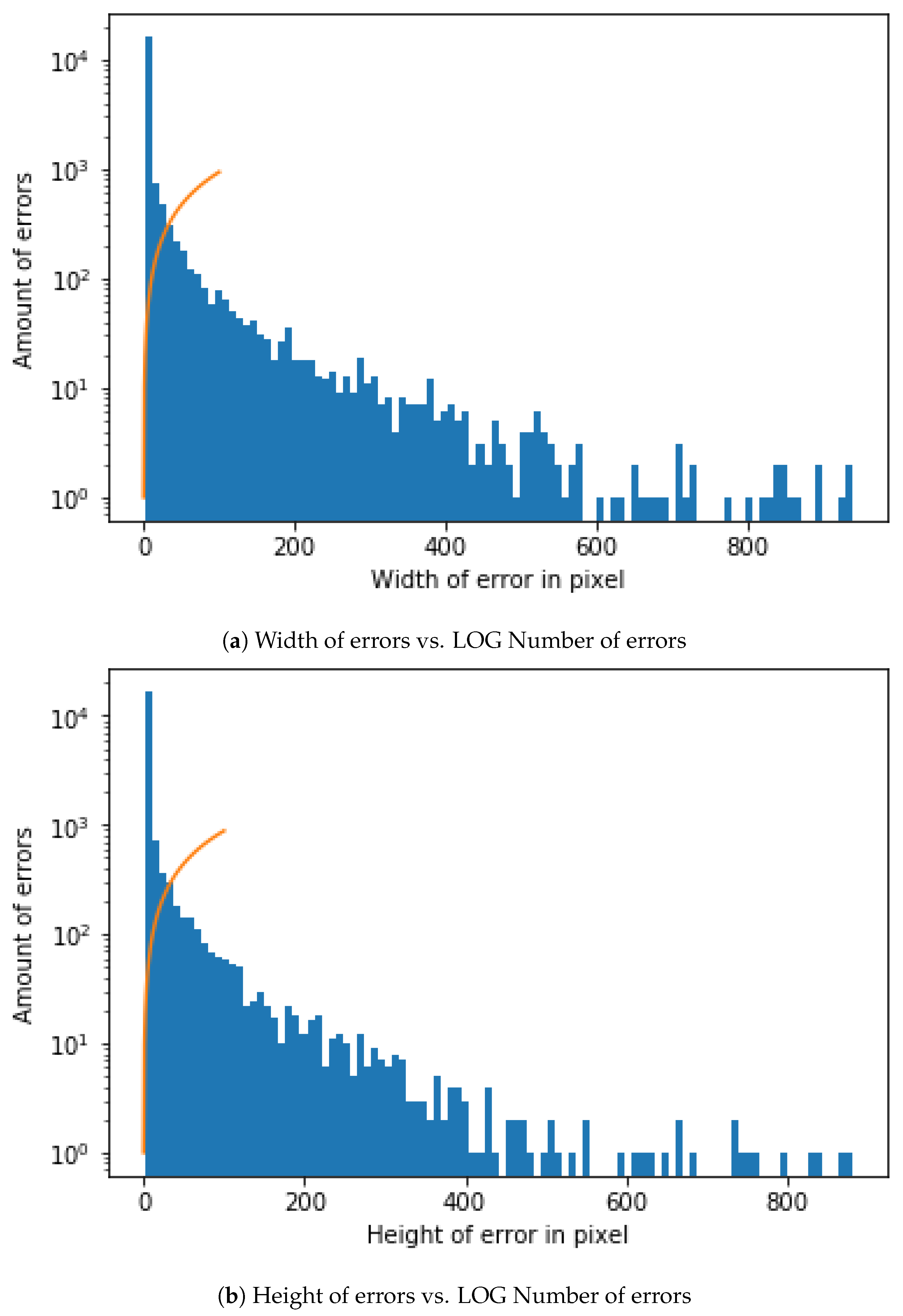
- Image Size for DNN Input and Convolutional Window SizeDue to the need for standardized input data, a decision needs to be made about which dimensions the input images should have. The first decision is the aspect ratio. The following decision should be how many pixels wide and high the input images should be. In order to get a first impression of the existing sizes, a short analysis of the previous manually confirmed errors is made. According to the data, the mean value of the width is slightly higher than that of the height. In the mean aspect ratio this gets even clearer with a mean aspect ratio of about 1.5. This is probably a result of some errors that are elongated by the rotation of the cylinder. The median aspect ratio is exactly at 1.0. Because the median describes a higher percentage of errors better this should also be the aspect ratio of the neural network input. As shown in the representation of the width and height of error in pixel against the LOG of the amount of errors Figure 6.As the size of the error also plays a role in the judgment of the errors, scaling operations should be reduced to a minimum. Due to the range of the sizes this is not always possible. The training time of the neural network would increase dramatically with large input sizes and small errors would mostly consist of OK-cylinder surface. Therefore a middle ground is needed so that most input images can be shown without much scaling or added OK-cylinder surface. A size in the middle would be 100 pixels. We therefore calculate the percentage of errors with the width smaller or equal to 100. The results show that about 90% of all errors have both the height and width below or equal to 100 and almost 74% have both the height and width below or equal to 10. One option would be to use an input size of 100 × 100.
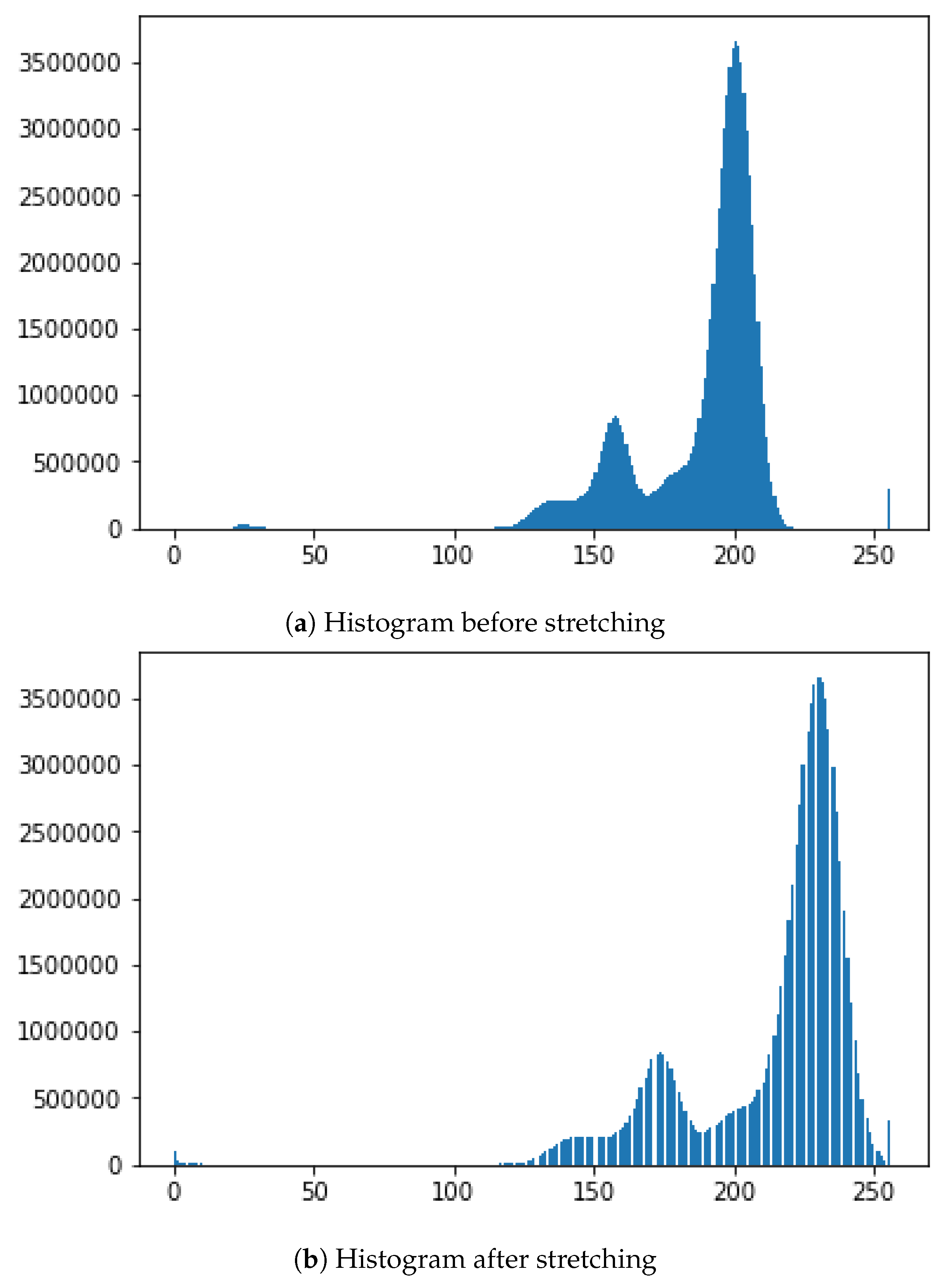
- Brightness AdjustmentTo get comparable data for all cylinder images, pre-processing is needed and is performed on the complete scan of a cylinder. From this scan multiple examples are taken. Because there can be slight deviations due to many influences during the recording of the cylinder surface, this can only be achieved by having a similar brightness for the cylinder surface and engraved parts. Another important point is that no essential information gets lost from the images and, that the brightness between the engraved and not engraved parts are comparable for all cylinder scans. Therefore a brightness stretch is needed but only few pixels are allowed to become the darkest or brightest pixels. Notwithstanding, the amount of pixel that become the darkest and brightest pixels ca not be set to a very low value because noise in the image data would result in big differences. In conclusion a low percentage of the pixels should be set as darkest and brightest. For example, the lowest and the highest percentage should each have a maximum of 0.5%. Figure 7 shows a stretching example for brightness adjustment for one image so that 0.5% of all pixels will have a value of 0 and 0.5% of all pixels will have the value of 255.
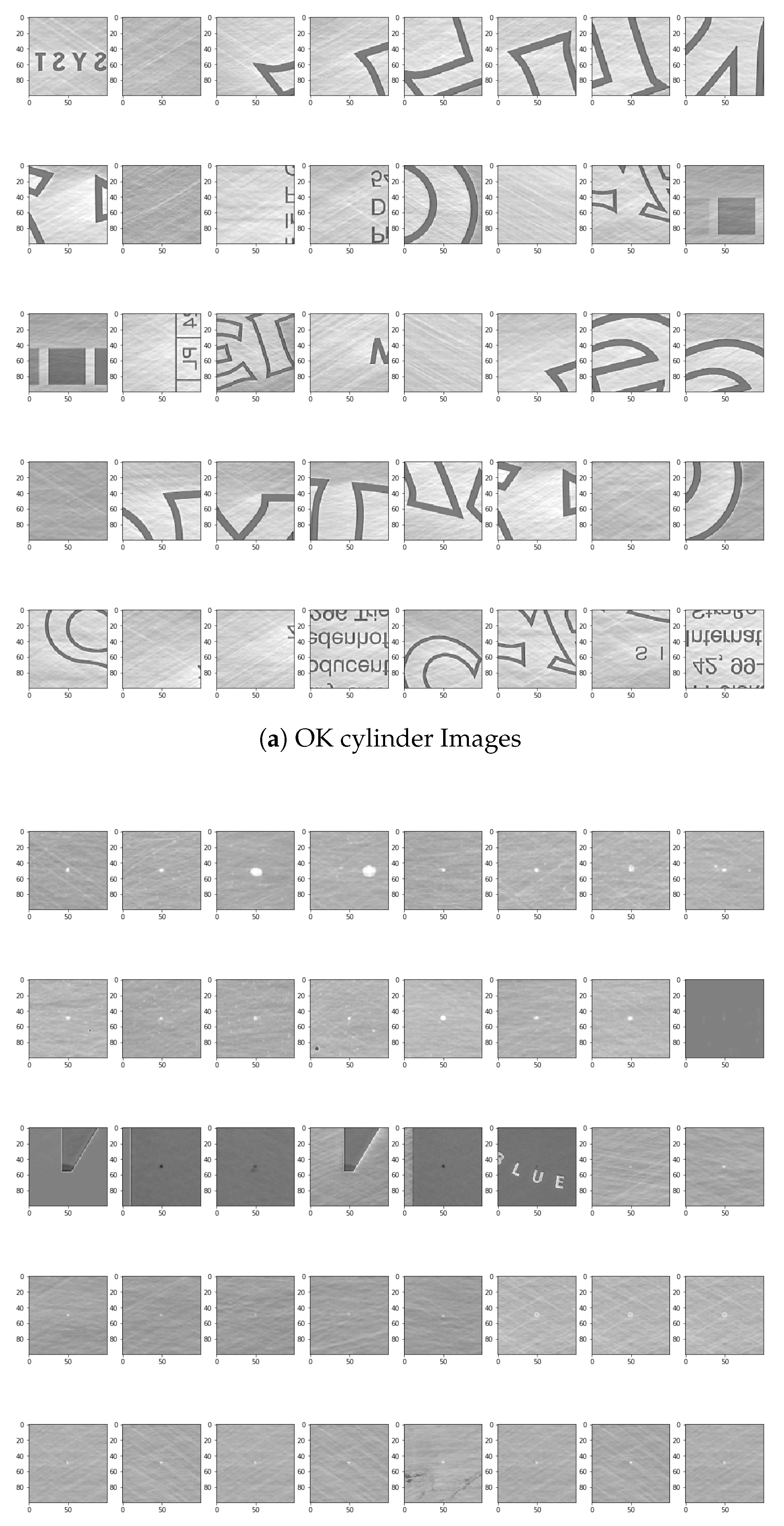
- Automatic selection and Dataset LabellingTo simplify the later steps, the images need to be cut from the original file and saved into two folders with examples that are OK-cylinder (Figure 8a) and examples that are not-OK-cylinder (Figure 8b). The great variety of patterns presented in the spectrum can be observed in the figures. The very nature of the process implies that each new product represents a new challenge for DNN, as it has probably never before been confronted with these images. For this reason, the errors may be of a very different nature. This implies a high complexity of solving the challenge of training and testing the DNN. Likewise, the different shades of black and grey, very difficult to appreciate with the naked eye when manually sorting the images, represent an added difficulty that must be resolved by DNN architecture.If errors are smaller in width or height than 100, the ROI gets increased to 100. If any size is bigger than 100 pixels is ignored. For the purpose of checking later on, the big input data is split into 100 × 100 parts. If any one of these is detected as an error, all are marked as an error. As shown in the Open Access Repository, there are multiple possible ways to handle the bigger data. Every example also has the actual and target data. There are different ways of using this data as input. One way is just using the actual data. A different option is to use the difference between the actual and expected data. The problem in both cases is that information gets lost. Better results have been achieved by using the differences. These get adjusted, so that the input data is in a range from [−1,1]. Once this is performed, and because a balanced dataset is important to train the neural network and the OK-cylinder examples far outnumber the not-OK-cylinder examples, an OK-cylinder example is only saved if a not-OK-cylinder example has been found previously.
3.1.3. Automatic Detection of Cylinder ErrorsUsing a DNN Soft Sensor
- Classification The first goal of this architecture is not to identify different objects inside of part of the images but to separate two classes (not-OK and OK images), where the main source of noise came from the illumination factor from the scanner lectures. Therefore, neither the so deep architectures nor the identity transference, which was the key for the ResNet [41] is needed in our case, and just few convolutions shall help identify convenient structural features to rely on.
- Performance. The proposed architecture is even more simplistic than the AlexNet [42] one, as we do not use five convolution layers but just three. The main reason is to look for a compromise between the number of parameters and the available dataset of images. Our architecture was always looking to be frugal in terms of resources, as it is expected to be a soft sensor, running in real time and having the inherent capability of retrain for reinforced learning, close to such real time constraint.
- Feature Extraction. The feature extraction is performed by a deep stack of alternatively fully connected convolutional and sub-sampling max pooling layers, the even numbered layers are for convolutions and the odd numbered layers are for max-pooling operations.
- -
- Convolution and ReLu (rectified linear unit) activated convolutional layers. Convolution operations, by means of activation functions, extract the features from the input information which are propagated to deeper level layers. A ReLu activation function is a function meant to zero out negative values. The ReLu activation function was first presented in AlexNet [42] and solves the vanishing gradient problem for training DNN.
- -
- Max pooling. Consists of extracting windows from the input feature maps and outputting the max value of each channel. It’s conceptually similar to convolution, except that instead of transforming local patches via a learned linear transformation (the convolution kernel), they are transformed via a max tensor operation.
- Classification. The classification is performed by fully connected activation layers [43]. Some examples of such models are LeNet [44], AlexNet [42], Network in Network [45], GoogLeNet [46,47,48], DenseNet [49].
- -
- Fully connected activation layers output a probability distribution over the output classes [25]. Because we are facing a binary classification problem and the output of our network is a probability, it is best to use the binary-crossentropy loss function. Crossentropy is a quantity from the field of Information Theory that measures the distance between probability distributions or, in this case, between the ground-truth distribution and the predictions. It is not the only viable choice: we could use, for instance, mean-squared-error. However, crossentropy is usually the best choice when dealing with models that output probabilities. Because we are attacking a binary-classification problem, we end the network with a single unit (a Dense layer of size 1) and a sigmoid activation. This unit will encode the probability that the network is looking at one class or the other [25].
3.1.4. Visualizing the Learned Features
4. Results and Discussion
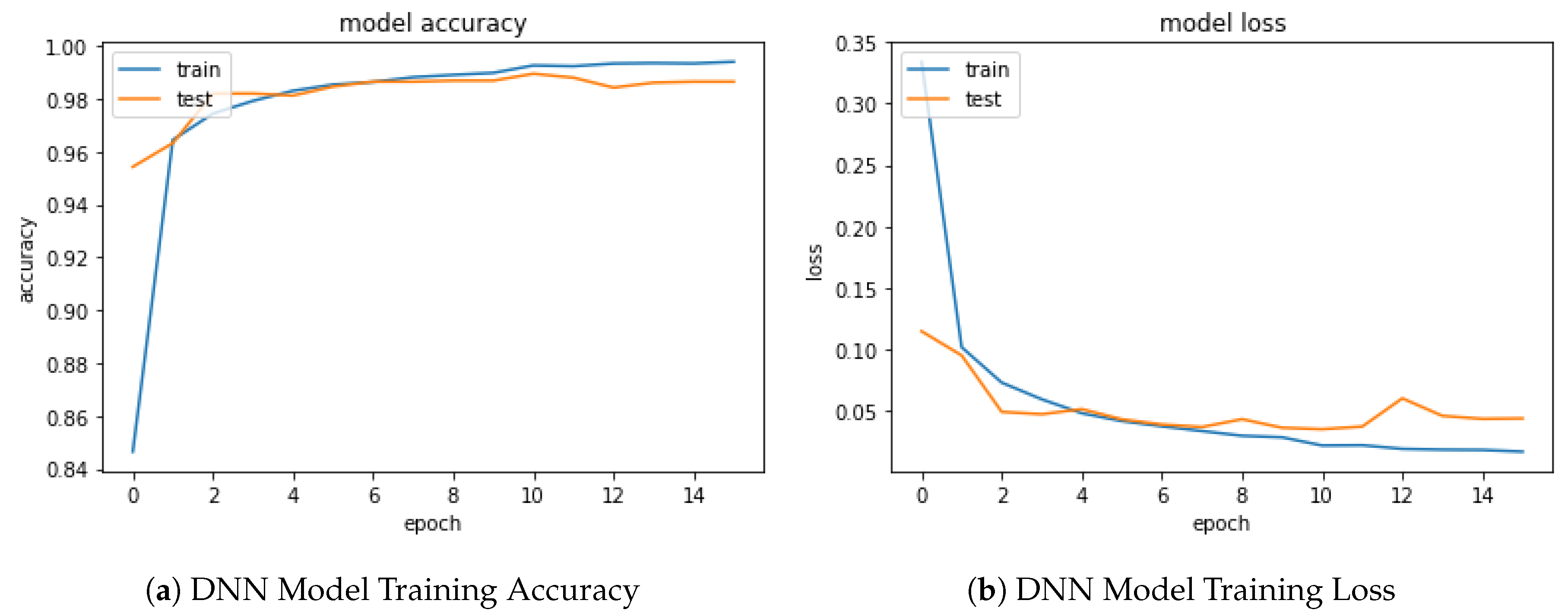
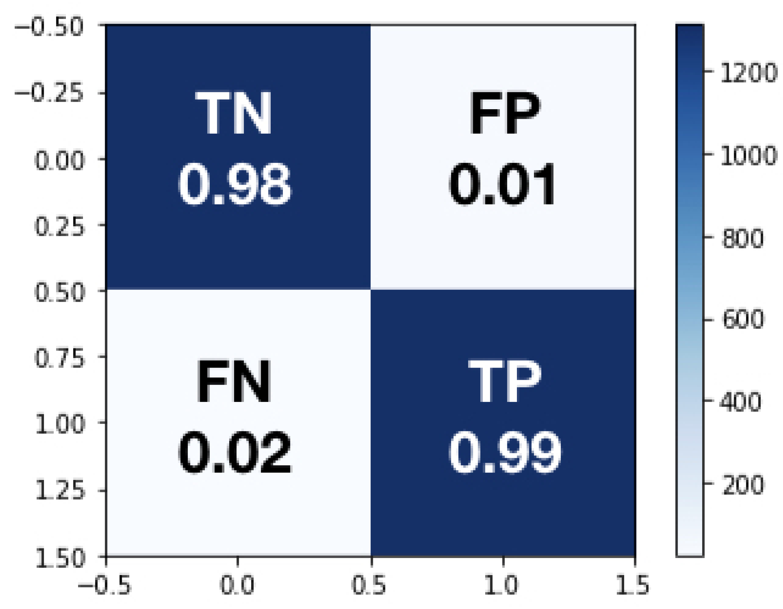
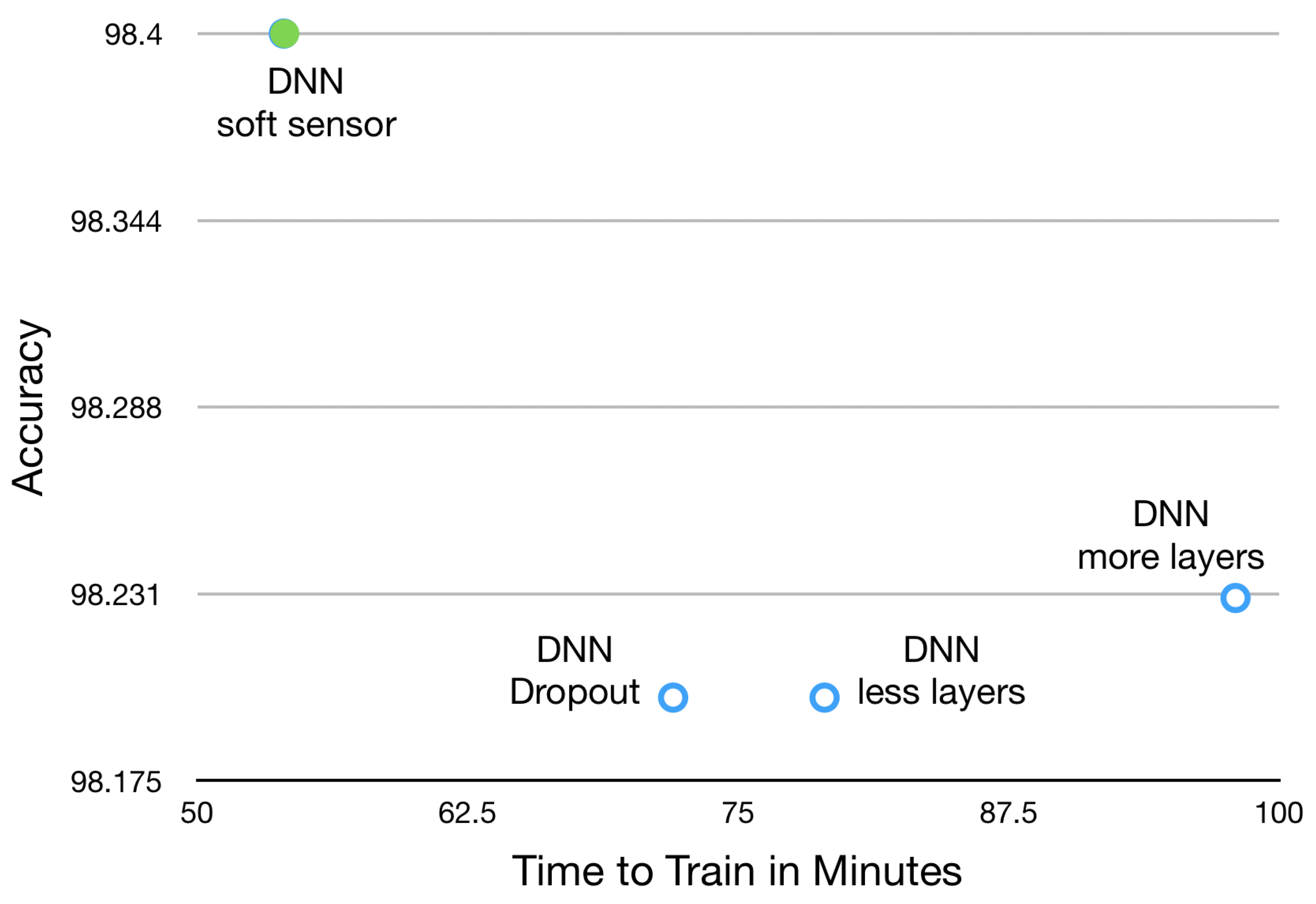
- Using the DNN fully automate OQC classification to predict the amount of errors a cylinder has.The DNN only provides a successful result 98.4% of the time. To be sure that the wrongly classified images are not big mistakes, human experts will review all possible errors. DNN has already had a positive influence on the workflow, as we know how many errors are very likely an error: DNN helps significantly in the planning of the next workflow step because it is known with a high probability if the cylinder needs to go to the correction department or if it is very likely that the product is an OK-cylinder.
- Showing the error probability to the operator that is currently deciding if it is an error or if it is not.This gives a hint to the operator, who can give feedback if there are relevant mistakes that were not predicted as mistakes. This can also help the operator to reduce the likelihood of missing an error. Once this soft sensor was integrated in production, OQC productivity, measured in hours per unit - time an operator spends in the OQC -, dramatically increased by 210% as decision about defects is made in an automatic way.
- Only showing possible errors that have been predicted by the DNN.In the last step, the DNN could completely filter out errors that are not relevant. This can also be used in multiple steps because it is possible to increase the threshold error probability for the possible error to be shown. At some point a threshold will have to be chosen taking into consideration the cost of checking a possible error and the cost of missing a error. This would completely eliminate the step of checking the errors and the confirmed errors would only be checked by the correction department.
5. Conclusions and Future Steps of Deep Learning in a Printing Industry 4.0 Context
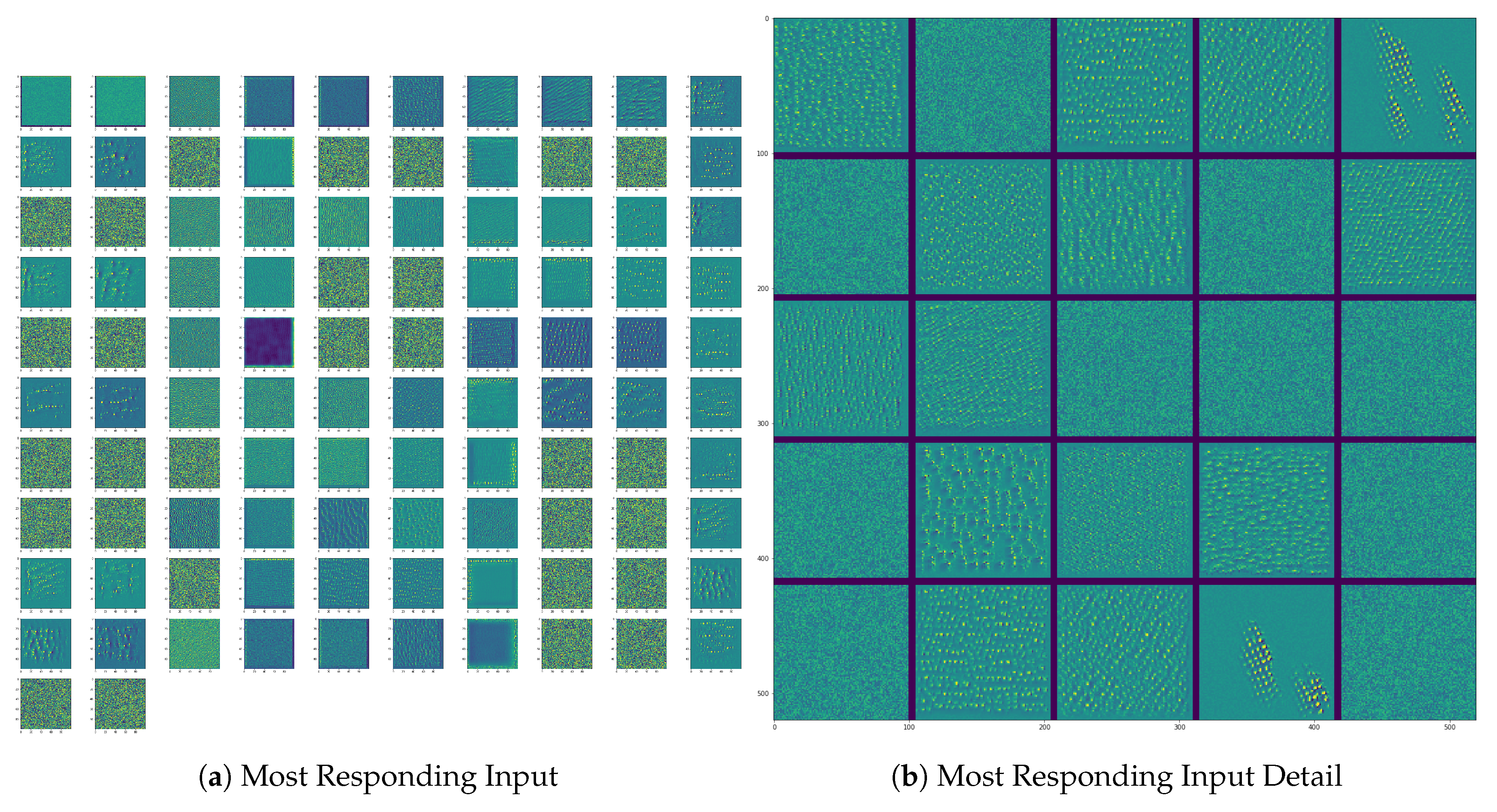
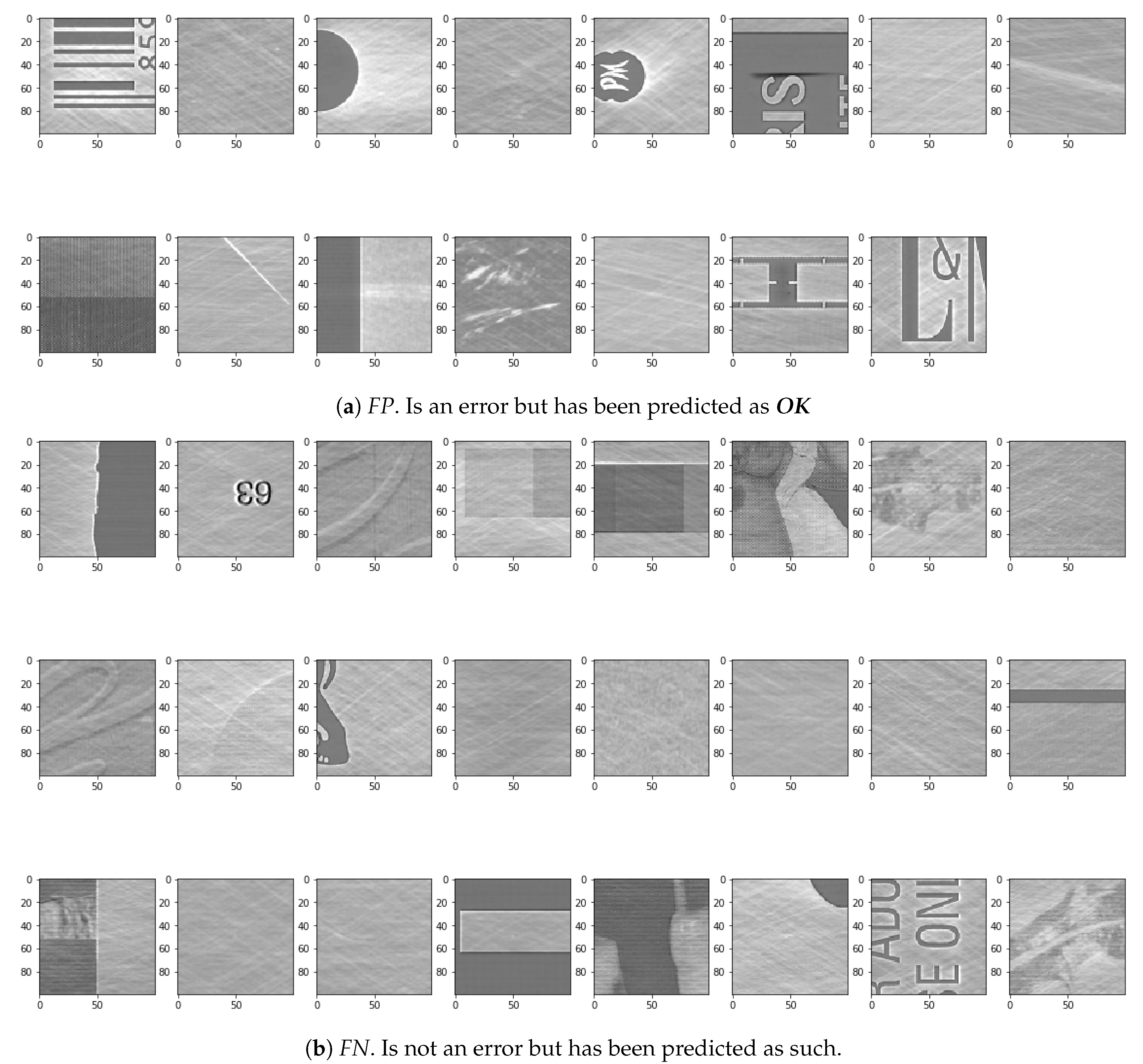
- Not-OKexamples that have been predicted asOK. Looking at the actual errors in the test data that have not been predicted as errors, as in Figure 15a, a few issues could be the cause of the wrong predictions. Some of the examples actually do not look like they are really not-OK. The cause of this could either be, that the input data was not labeled correctly or that the error really is not highly visible in the image.
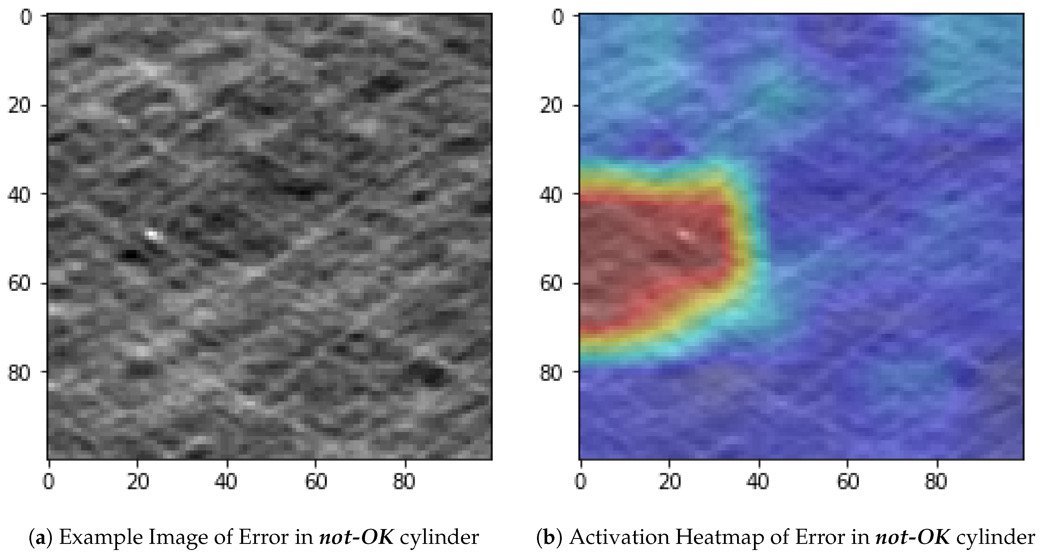
- OKexamples that have been predicted asnot-OK. After looking at the visualization of the DNN, it gets clear that the main focus for finding mistakes is looking for extreme edges. These can be seen in a lot of the wrongly classified examples. Especially the first two examples seen in Figure 15b have some extreme edges that are a result of a slight misalignment of the images in the pre-processing. Therefore the image registration in the pre-processing part between the original and the recording of the cylinder surface needs to be improved.
- Deep Learning at a shopfloor level shall impact quality, reliability and cost.At the shopfloor level, this paper has shown an example of how deep learning increases the effectiveness and efficiency of process control aimed at achieving better quality (e.g., with OQC) and lower costs, allowing self-correction of processes by means of shorter and more accurate quality feedback loops. This intelligence integrated in the value streams will allow many humans and machines to co-exist in a way in which artificial intelligence will complement in many aspects. In the future, significant challenges will still be encountered in the generation and collection of data from the shopfloor.The main challenge towards a fully automated solution is currently getting the Python DNN integrated into the C++ cLynx program. After this is successfully completed, a testing phase with the cLynx users is planned. If the results are satisfactory, the complete automatic process will be started. If the results are not satisfying, further steps have to be taken so as to improve the DNN further.
- Deep Learning at a supply chain level shall impact lead time and on-time delivery.At a higher level of supply chain, producing only what the customer needs, when it needs it, in the required quality, the integration of deep learning technology will allow not only the systematic improvement of complex value chains, but a better use and exploitation of resources, thus reducing the environmental impact of industrial processes 4.0.
- Deep Learning at a strategic level shall impact sustainable growth.At a more strategic level, customers and suppliers will be able to reach new levels of transparency and traceability on the quality and efficiency of the processes, which will generate new business opportunities for both, generating new products and services and cooperation opportunities in a cyber–physical environment. In a world of limited resources, increasing business volume can only be achieved by increasing the depth of integrated intelligence capable of successfully handling the emerging complexity in value streams.
Author Contributions
Funding
Acknowledgments
Conflicts of Interest
Abbreviations
| IIoT | Industrial Internet of Things |
| OQC | Optical Quality Control |
| DNN | Deep Neural Networks |
| GPU | Graphic Process Unit |
| RAM | Random Access Memory |
References
- Ustundag, A.; Cevikcan, E. Industry 4.0: Managing The Digital Transformation; Springer Series in Advanced Manufacturing; Springer: Cham, Switzerland, 2018. [Google Scholar]
- Davis, J.; Edgar, T.; Porter, J.; Bernaden, J.; Sarli, M. Smart manufacturing, manufacturing intelligence and demand-dynamic performance. Comput. Chem. Eng. 2012, 47, 145–156. [Google Scholar] [CrossRef]
- Li, L. China’s manufacturing locus in 2025: With a comparison of ‘Made-in-China 2025’ and ‘Industry 4.0’. Technol. Forecast. Soc. Chang. 2018, 135, 66–74. [Google Scholar] [CrossRef]
- Shiroishi, Y.; Uchiyama, K.; Suzuki, N. Society 5.0: For Human Security and Well-Being. Computer 2018, 51, 91–95. [Google Scholar] [CrossRef]
- Womack, J.; Roos, D. The Machine That Changed the World; Harper Perennial: New York, NY, USA, 1990. [Google Scholar]
- Takeda, H. Intelligent Automation Textbook; Nikkan Kogyo Shimbun: Tokyo, Japan, 2009. [Google Scholar]
- Nakabo, Y. Considering the competition and cooperation areas surrounding Industry 4.0. What will IoT automate. J-Stage Top. Meas. Contr. 2015, 54, 912–917. [Google Scholar] [CrossRef]
- Kuwahara, S. About factory automation and IoT, AI utilization by intelligent robot. J-Stage Top. Syst. Contr. Inf. 2017, 61, 101–106. [Google Scholar] [CrossRef]
- Villalba-Diez, J.; Ordieres-Mere, J. Improving manufacturing operational performance by standardizing process management. IEEE Trans. Eng. Manag. 2015, 62, 351–360. [Google Scholar] [CrossRef]
- Villalba-Diez, J.; Ordieres-Mere, J.; Chudzick, H.; Lopez-Rojo, P. NEMAWASHI: Attaining Value Stream alignment within Complex Organizational Networks. Procedia CIRP 2015, 7, 134–139. [Google Scholar] [CrossRef]
- Jimenez, P.; Villalba-Diez, J.; Ordieres-Mere, J. HOSHIN KANRI Visualization with Neo4j. Empowering Leaders to Operationalize Lean Structural Networks. PROCEDIA CIRP 2016, 55, 284–289. [Google Scholar] [CrossRef]
- Villalba-Diez, J. The HOSHIN KANRI FOREST. Lean Strategic Organizational Design, 1st ed.; CRC Press, Taylor and Francis Group LLC: Boca Raton, FL, USA, 2017. [Google Scholar]
- Villalba-Diez, J. The Lean Brain Theory. Complex Networked Lean Strategic Organizational Design; CRC Press, Taylor and Francis Group LLC: Boca Raton, FL, USA, 2017. [Google Scholar]
- Womack, J.; Jones, D. Introduction. In Lean Thinking, 2nd ed.; Simon & Schuster: New York, NY, USA, 2003; p. 4. [Google Scholar]
- Arai, T.; Osumi, H.; Ohashi, K.; Makino, H. Production Automation Committee Report: 50 years of automation technology. J-Stage Top. Precis. Eng. J. 2018, 84, 817–820. [Google Scholar] [CrossRef][Green Version]
- Manikandan, V.S.; Sidhureddy, B.; Thiruppathi, A.R.; Chen, A. Sensitive Electrochemical Detection of Caffeic Acid in Wine Based on Fluorine-Doped Graphene Oxide. Sensors 2019, 19, 1604. [Google Scholar] [CrossRef]
- Garcia Plaza, E.; Nunez Lopez, P.J.; Beamud Gonzalez, E.M. Multi-Sensor Data Fusion for Real-Time Surface Quality Control in Automated Machining Systems. Sensors 2018, 18, 4381. [Google Scholar] [CrossRef] [PubMed]
- Han, L.; Cheng, X.; Li, Z.; Zhong, K.; Shi, Y.; Jiang, H. A Robot-Driven 3D Shape Measurement System for Automatic Quality Inspection of Thermal Objects on a Forging Production Line. Sensors 2018, 18, 4368. [Google Scholar] [CrossRef] [PubMed]
- Weimer, D.; Scholz-Reiter, B.; Shpitalni, M. Design of deep convolutional neural network architectures for automated feature extraction in industrial inspection. CIRP Annals 2016, 65, 417–420. [Google Scholar] [CrossRef]
- Xie, X. A Review of Recent Advances in Surface Defect Detection Using Texture Analysis Techniques. Electron. Lett. Comput. Vision Image Ana. 2008, 7, 1–22. [Google Scholar] [CrossRef]
- Scholz-Reiter, B.; Weimer, D.; Thamer, H. Automated Surface Inspection of Cold-Formed MicroPart. CIRP Ann. Manuf. Technol. 2012, 61, 531–534. [Google Scholar] [CrossRef]
- Rani, S.; Baral, A.; Bijender, K.; Saini, M. Quality control during laser cut rotogravure cylinder manufacturing processes. Int. J. Sci. Eng. Comput. Technol. 2015, 5, 70–73. [Google Scholar]
- LeCun, Y.; Bengio, Y.; Hinton, G. Deep learning. Nature 2015, 521, 436–444. [Google Scholar] [CrossRef] [PubMed]
- Jia, Y.; Shelhamer, E.; Donahue, J.; Karayev, S.; Long, J.; Girshick, R.; Guadarrama, S.; Darrell, T. Caffe: Convolutional Architecture for Fast Feature Embedding. ACM Multimedia 2014, 675–678. [Google Scholar]
- Chollet, F. Deep Learning with Python; Manning Publications Co.: Shelter Island, NY, USA, 2018. [Google Scholar]
- Lin, T.; RoyChowdhury, A.; Maji, S. Bilinear CNN Models for Fine-Grained Visual Recognition. In Proceedings of the 2015 IEEE International Conference on Computer Vision (ICCV), Santiago, Chile, 7–13 December 2015; pp. 1449–1457. [Google Scholar] [CrossRef]
- Miskuf, M.; Zolotova, I. Comparison between multi-class classifiers and deep learning with focus on industry 4.0. In Proceedings of the 2016 Cybernetics & Informatics (K&I), Levoca, Slovakia, 2–5 February 2016. [Google Scholar]
- Zheng, X.; Wang, M.; Ordieres-Mere, J. Comparison of Data Preprocessing Approaches for Applying Deep Learning to Human Activity Recognition in the Context of Industry 4.0. Sensors 2018, 2146, 2146. [Google Scholar] [CrossRef]
- Aviles-Cruz, C.; Ferreyra-Ramirez, A.; Zuniga-Lopez, A.; Villegas-Cortez, J. Coarse-Fine Convolutional Deep-Learning Strategy for Human Activity Recognition. Sensors 2019, 19, 1556. [Google Scholar] [CrossRef]
- Zhe, L.; Wang, K.S. Intelligent predictive maintenance for fault diagnosis and prognosis in machine centers: Industry 4.0 scenario. Adv. Manuf. 2017, 5, 377–387. [Google Scholar]
- Deutsch, J.; He, D. Using Deep Learning-Based Approach to Predict Remaining Useful Life of Rotating Components. IEEE Trans. Syst. Man Cybern. Syst. 2018, 48, 11–20. [Google Scholar] [CrossRef]
- Shanmugamani, R. (Ed.) Deep Learning for Computer Vision; Packt Publishing-ebooks Account: Birmingham, UK, 2018. [Google Scholar]
- Wang, T.; Chen, Y.; Qiao, M.; Snoussi, H. A fast and robust convolutional neural network-based defect detection model in product quality control. Int. J. Adv. Manuf. Technol. 2018, 94, 3465–3471. [Google Scholar] [CrossRef]
- He, M.; He, D. Deep Learning Based Approach for Bearing Fault Diagnosis. IEEE Trans. Ind. App. 2017, 53, 3057–3065. [Google Scholar] [CrossRef]
- Imai, M. KAIZEN: The Key to Japan’s Competitive Success; McGraw-Hill Higher Education: New York, NY, USA, 1986. [Google Scholar]
- Schmidt, D. Available online: https://patentscope.wipo.int/search/de/detail.jsf;jsessionid=F4DFD8F2D86BB91896D53B4AB97E84A1.wapp1nC?docId=WO2018166551&recNum=871&office=&queryString=&prevFilter=&sortOption=Ver%C3%B6ffentlichungsdatum+ab&maxRec=70951352 (accessed on 15 September 2019).
- Hinton, G.; Osindero, S.; Teh, Y. A fast learning algorithm for deep belief nets. Neural Comput. 2006, 18, 1527–1554. [Google Scholar] [CrossRef]
- Zhang, K.; Zuo, W.; Gu, S.; Zhang, L. Learning Deep CNN Denoiser Prior for Image Restoration. In Proceedings of the 2017 IEEE Conference on Computer Vision and Pattern Recognition (CVPR), Honolulu, HI, USA, 21–26 July 2017; pp. 2808–2817. [Google Scholar] [CrossRef]
- Zhang, K.; Zuo, W.; Chen, Y.; Meng, D.; Zhang, L. Beyond a Gaussian Denoiser: Residual Learning of Deep CNN for Image Denoising. IEEE Trans. Image Process. 2017, 26, 3142–3155. [Google Scholar] [CrossRef] [PubMed]
- van Rossum, G. Python Tutorial; Technical Report CS-R9526; Computer Science/Department of Algorithmics and Architecture: Amsterdam, The Netherlands, 1995. [Google Scholar]
- He, K.; Zhang, X.; Ren, S.; Sun, J. Deep Residual Learning for Image Recognition. arXiv 2015, arXiv:1512.03385. [Google Scholar]
- Krizhevsky, A.; Sutskever, L.; Hinton, G. Imagenet classification with deep convolutional neural networks. In Proceedings of the 25th International Conference on Neural Information Processing Systems, Lake Tahoe, NV, USA, 3–6 December 2012; pp. 1106–1114. [Google Scholar]
- Alom, M.Z.; Taha, T.M.; Yakopcic, C.; Westberg, S.; Sidike, P.; Nasrin, M.S.; Hasan, M.; Van Essen, B.C.; Awwal, A.A.S.; Asari, V.K. A State-of-the-Art Survey on Deep Learning Theory and Architectures. Electronics 2019, 8, 292. [Google Scholar] [CrossRef]
- Lecun, Y.; Bottou, L.; Bengio, Y.; Haffner, P. Gradient-based learning applied to document recognition. Proc. IEEE 1998, 86, 2278–2324. [Google Scholar] [CrossRef]
- Lin, M.; Chen, Q.; Yan, S. Network In Network. arXiv 2013, arXiv:1312.4400. [Google Scholar]
- Szegedy, C.; Liu, W.; Jia, Y.; Sermanet, P.; Reed, S.; Anguelov, D.; Erhan, D.; Vanhoucke, V.; Rabinovich, A. Going deeper with convolutions. In Proceedings of the 2015 IEEE Conference on Computer Vision and Pattern Recognition (CVPR), Bosto, MA, USA, 7–12 June 2015; pp. 1–9. [Google Scholar] [CrossRef]
- Szegedy, C.; Vanhoucke, V.; Ioffe, S.; Shlens, J.; Wojna, Z. Rethinking the Inception Architecture for Computer Vision. arXiv 2015, arXiv:1512.00567. [Google Scholar]
- Szegedy, C.; Ioffe, S.; Vanhoucke, C.; Alemi, A. Inception-v4, Inception-ResNet and the Impact of Residual Connections on Learning. arXiv 2016, arXiv:1602.07261. [Google Scholar]
- Huang, G.; Liu, Z.; Maaten, L.v.d.; Weinberger, K.Q. Densely Connected Convolutional Networks. In Proceedings of the 2017 IEEE Conference on Computer Vision and Pattern Recognition (CVPR), Honolulu, HI, USA, 21–26 July 2017; pp. 2261–2269. [Google Scholar]


| Stage | Description of Improvement |
|---|---|
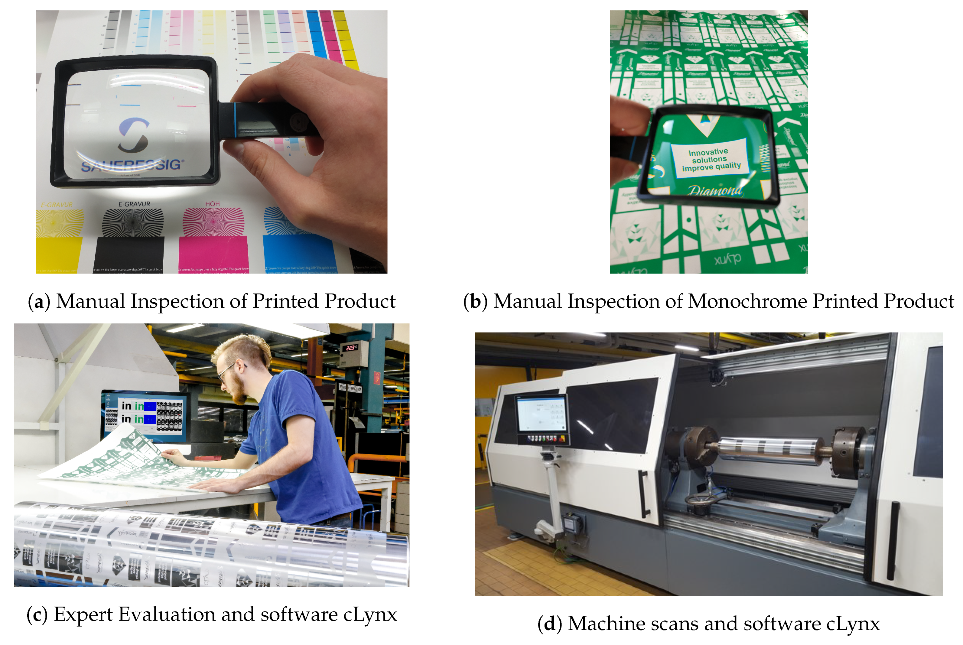
| Manual Inspection of Printed Product (Figure 2a) | In the first stage all cylinders of an order were printed together. Due to the processes used producing gravure cylinders, mistakes like holes in the cylinder are almost inevitable. To check the quality of the gravure cylinders, all the cylinders of one order are generally printed together and the resulting print checked manually with the help of a magnifying glass. To do this the approximate color of each individual cylinder must be mixed and all cylinders are printed one after the other on one substrate. On average this can be 5–10 cylinders or colours in one job. The big disadvantage is that all cylinders of a job must already be present. Thus, a one-piece flow is not possible. In addition, a lot of time is spent mixing the colours. As a direct comparison with the expected data was very difficult, the search for errors was focused on the most common errors that can happen during the production of an engraved printing cylinder. The coppering of the cylinder is a galvanic process, therefore it is possible that the cylinder has holes that also print. Another common mistake in the production of engraved printing cylinders is that parts that should print do not print. This can have different causes. Most of them can be traced back to problems during the engraving of the cylinder. To find these errors without a comparison to the expected data a search for irregularities in the carried out. As there are a lot of issues that had to be checked it was quite an ergonomically-challenging job, where some mistakes were not caught during the check. |
| Manual Inspection of Individual Color Printed Product (Figure 2b) | In the second stage the cylinders were all printed individually in the same (green) colour. In an attempt to further improve the quality control of each individual cylinder, the cylinder can also be printed itself. This impression was also checked manually with a magnifying glass by process experts. This has the advantage that there is no need to wait for the other cylinders of a job and no need to mix colours. However, the manual reading of the prints takes longer because there is one print for every cylinder of an order (5–10 cylinders) and not only one print for one order. Although this increased process reliability because process mistakes were directly tested on the product, the ergonomic weaknesses of the OQC process based on human experts could not be eliminated with this new improvement. |
| Evaluation of Errors by an Expert with aid of patented Software cLynx (Figure 2c) | This was then solved by the third stage: the digital scanning of the cylinder supported by the patented cLynx software (DE102017105704B3) [36]. To improve the quality and automate the process, a software named cLynx was developed to automatically compare the scanned file with the engraving file. The invention relates to a method for checking a printing form, in particular a gravure cylinder, for errors in an engraving printing form. A press proof of a cylinder gets printed and scanned using a high-resolution scanner. To compare the scans with the engraving file, a sequence of registration steps are performed. As a result the scans are matched with the engraving file. The differences between the two files are subject to a threshold in order to present the operator with a series of possible errors. As a result, the complexity of checking the entire print is reduced to a few possible errors that are checked by the operator. Since most of the work of troubleshooting was done by scanning + software, only the most conspicuous spots found by the software had to be evaluated by an expert. |
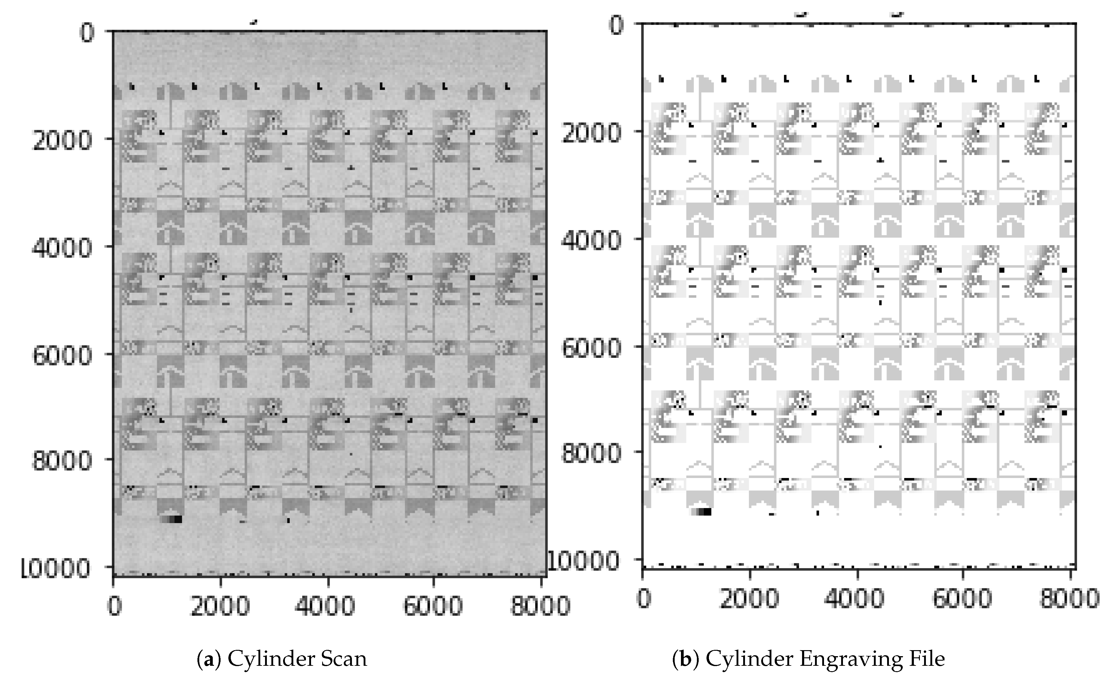
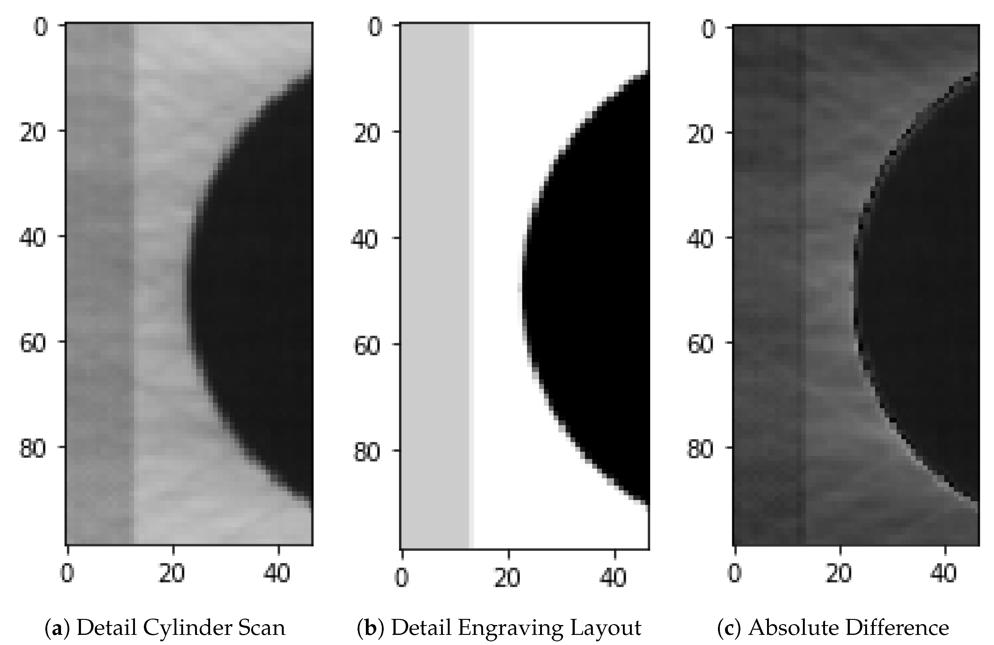
| Machine scans the cylinder and integrates the software cLynx (Figure 2d) | In the fourth stage, the entire printing process is omitted, as the cylinder surface is recorded directly with a camera within a cylinder scanning machine. To further reduce the cost of quality inspection, there is a need to check the cylinder without having to print it. To scan the surface of the cylinder a machine was built with a high-resolution line camera that scans the rotating cylinder at an approximate current speed of 1 meter/second. Because the scanning itself takes a minor portion of the processing time, this speed could actually be increased with a brighter LED lamp. After every movement a picture is taken, resulting in a flat image of the cylinder (Figure 3a). The main principles stay the same as with the scanned prints, as two complete recordings of the cylinder are made. These get matched to the engraving file and possible errors are presented to the operator using fixed thresholds (Figure 3b). This is done by automatically selecting areas around possible errors and calculating the absolute difference between the cylinder scan and the layout engraving file as shown in Figure 4. This significantly shortens the inspection time. However, the most prominent areas still have to be evaluated manually by the employee. For this reason, another fifth step towards a fully automated process is desired. |
| Layer Size | Layer Name | Layer Description and Rationale behind the Choice |
|---|---|---|
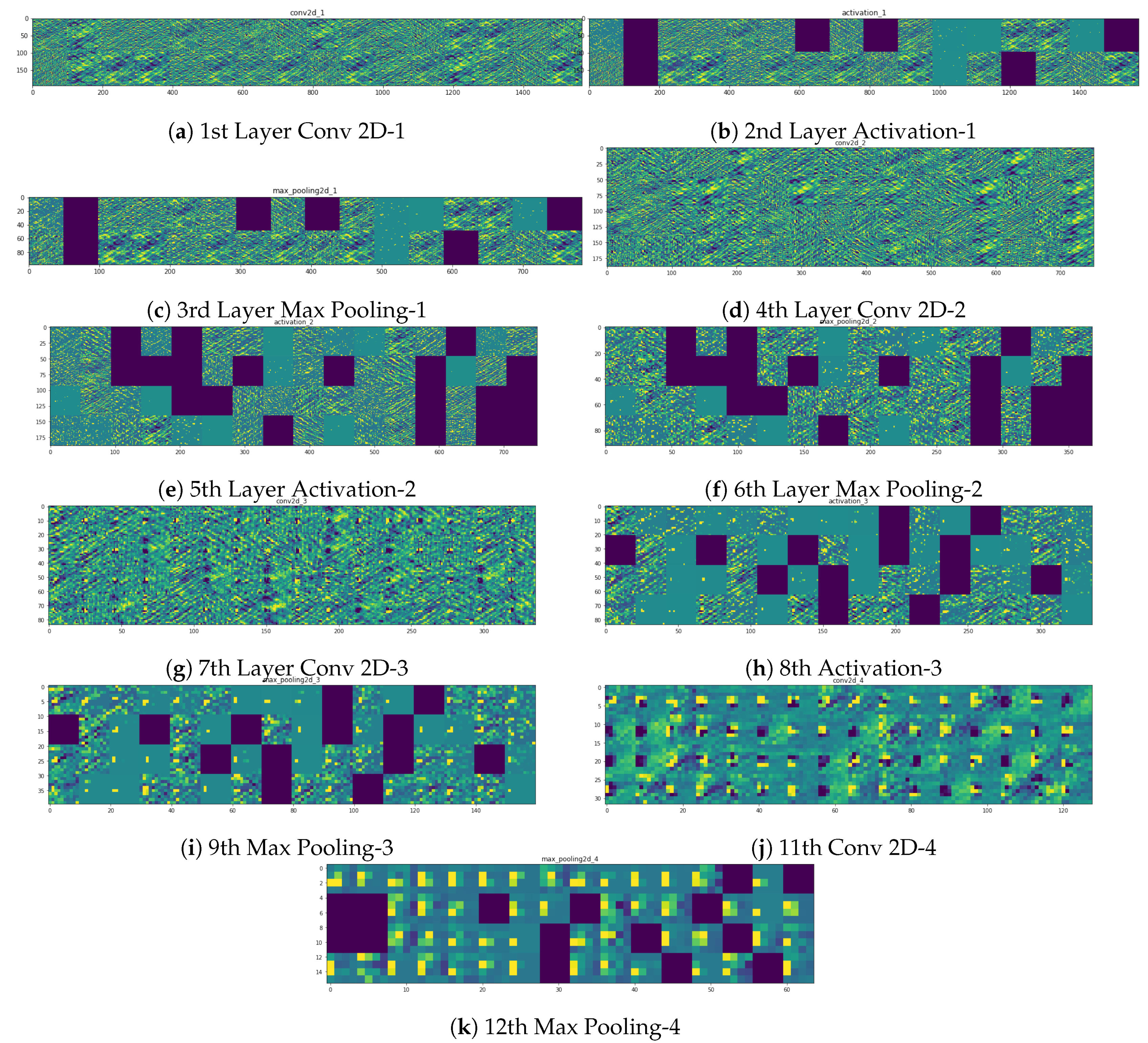
| (98, 98, 32) | conv2d 1 activation 1 (relu) | This is the first convolutional layer of the network. As observed in Figure 12 this layer mainly finds edges in the input image. In order to keep the values in check, an activation function is needed after each convolutional layer. |
| (49, 49, 32) | max pooling2d 1 | In order to reduce the complexity of the convoluted result a max pooling layer is used. Only the maximum in this case of a 2 × 2 pixel window is chosen. |
| (47, 47, 64) | conv2d 2 activation 2 (relu) | In the second convolutional layer the results describe more complex forms as is visible in Figure 12. In order to keep the values in check, an activation function is needed after each convolutional layer. |
| (23, 23, 64) | max pooling2d 2 | As with the previous max pooling layer this layer is used to reduce the complexity of the convoluted result. |
| (21, 21, 64) | conv2d 3 activation 3 (relu) | In the third convolutional layer resulting features are even more complex. In order to keep the values in check, an activation function is needed after each convolutional layer. |
| (10, 10, 64) | max pooling2d 3 | As with the previous max pooling layer this layer is used to reduce the complexity of the convoluted result. |
| (8, 8, 32) | conv2d 4 activation 4 (relu) | This is the final convolutional layer with the most complex features. In order to keep the values in check, an activation function is needed after each convolutional layer. |
| (4, 4, 32) | max pooling2d 4 | As with the previous max pooling layer this layer is used to reduce the complexity of the convoluted result. |
| (512) | flatten 1 | The flatten layer is used to flatten the previous 3 dimensional tensor to 1 dimension. |
| (64) | dense 1 activation 5 (relu) | To further reduce the complexity we use a fully connected layer. Before the final connection takes place the relu function is used to zero out the negative results. |
| (1) | dense 2 activation 6 (sigmoid) | As the probability of the input image being an error is wanted, the sigmoid function is needed to transform the input value into a probability [0–1]. |
© 2019 by the authors. Licensee MDPI, Basel, Switzerland. This article is an open access article distributed under the terms and conditions of the Creative Commons Attribution (CC BY) license (http://creativecommons.org/licenses/by/4.0/).
Share and Cite
Villalba-Diez, J.; Schmidt, D.; Gevers, R.; Ordieres-Meré, J.; Buchwitz, M.; Wellbrock, W. Deep Learning for Industrial Computer Vision Quality Control in the Printing Industry 4.0. Sensors 2019, 19, 3987. https://doi.org/10.3390/s19183987
Villalba-Diez J, Schmidt D, Gevers R, Ordieres-Meré J, Buchwitz M, Wellbrock W. Deep Learning for Industrial Computer Vision Quality Control in the Printing Industry 4.0. Sensors. 2019; 19(18):3987. https://doi.org/10.3390/s19183987
Chicago/Turabian StyleVillalba-Diez, Javier, Daniel Schmidt, Roman Gevers, Joaquín Ordieres-Meré, Martin Buchwitz, and Wanja Wellbrock. 2019. "Deep Learning for Industrial Computer Vision Quality Control in the Printing Industry 4.0" Sensors 19, no. 18: 3987. https://doi.org/10.3390/s19183987
APA StyleVillalba-Diez, J., Schmidt, D., Gevers, R., Ordieres-Meré, J., Buchwitz, M., & Wellbrock, W. (2019). Deep Learning for Industrial Computer Vision Quality Control in the Printing Industry 4.0. Sensors, 19(18), 3987. https://doi.org/10.3390/s19183987


