Promising Generative Adversarial Network Based Sinogram Inpainting Method for Ultra-Limited-Angle Computed Tomography Imaging

 , ,
, ,
Abstract
1. Introduction
2. Methods
2.1. CT Imaging Theory
2.2. Network Design
2.3. Image Reconstruction from Estimated Sinogram
3. Experimental Design
3.1. Experimental Data and Training Configuration
3.1.1. Digital CT Image Study
3.1.2. Anthropomorphic Head Phantom Study
3.2. Performance Evaluation
3.3. Comparison Methods
4. Results
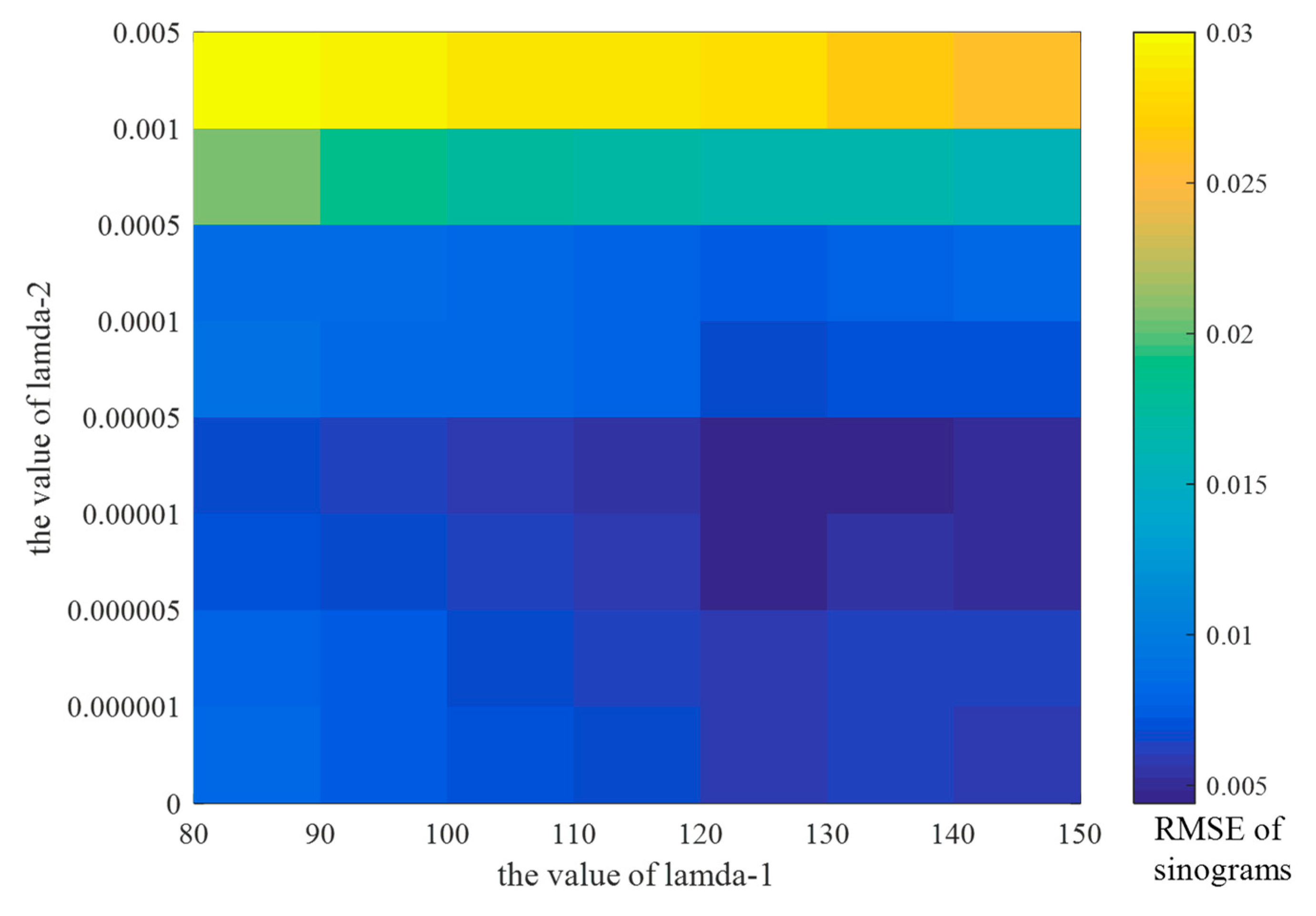
4.1. Parameter Selection of Loss Function
4.2. Simulation Study
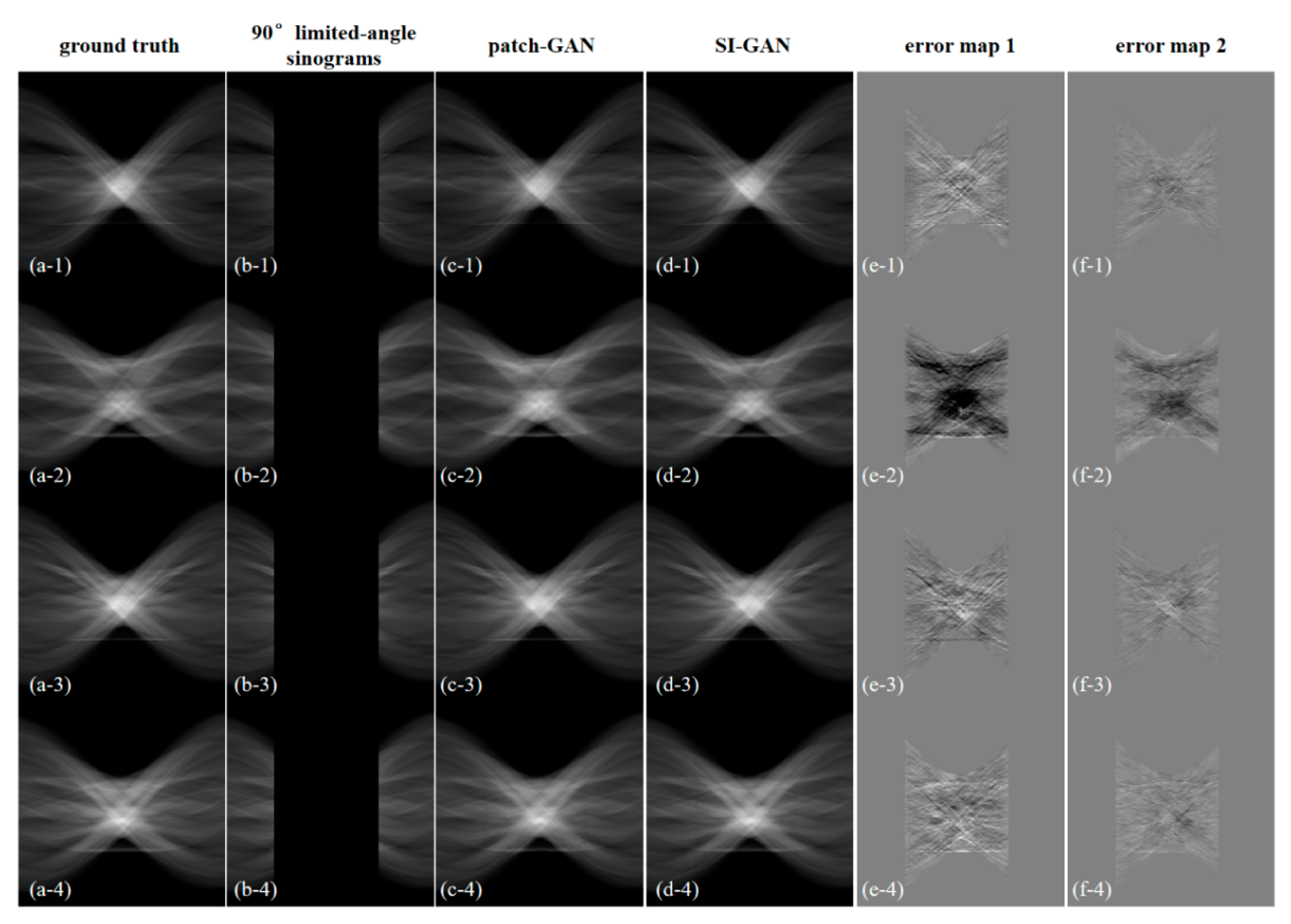
4.2.1. Sinogram Inpainting Test One (90° Scanning Angles)
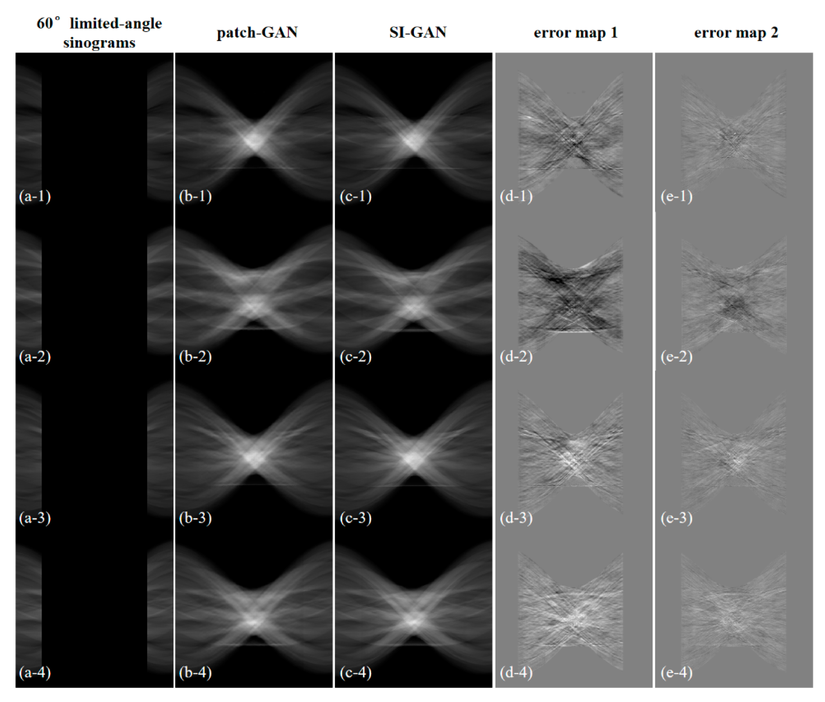
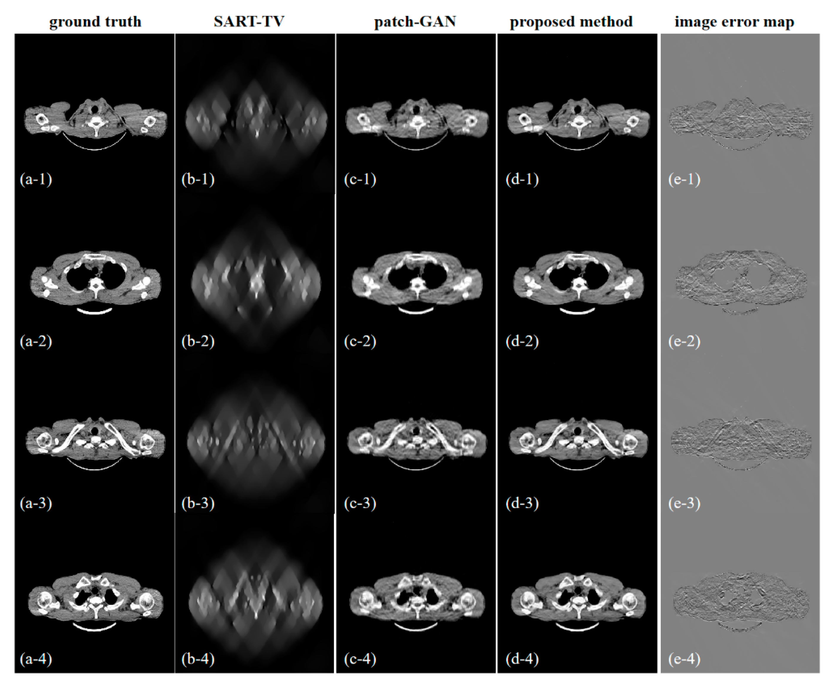
4.2.2. Sinogram Inpainting Test Two (60° Scanning Angles)
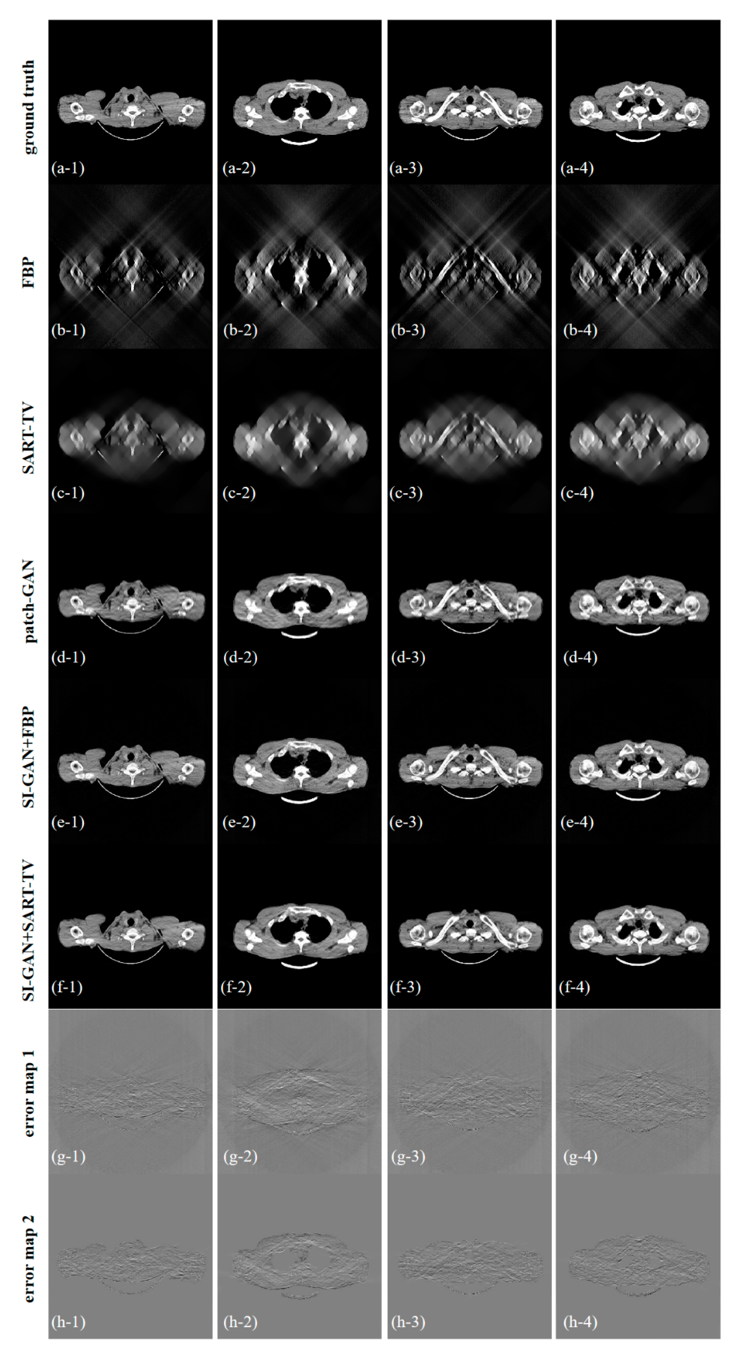
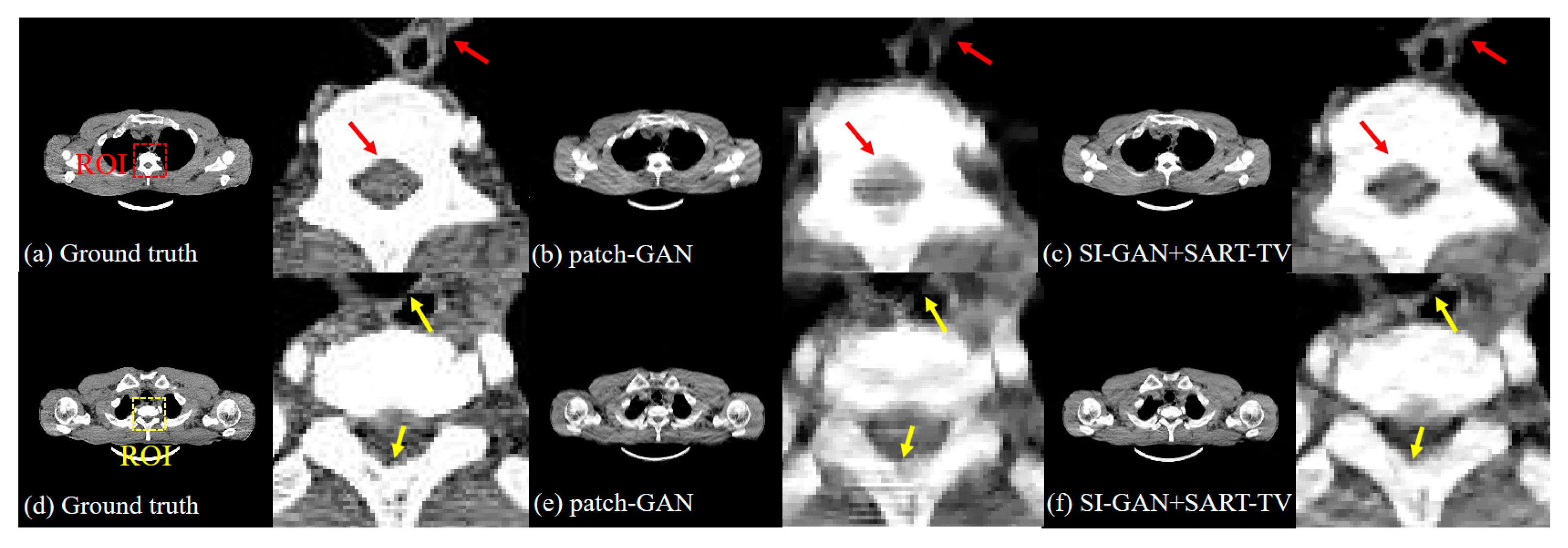
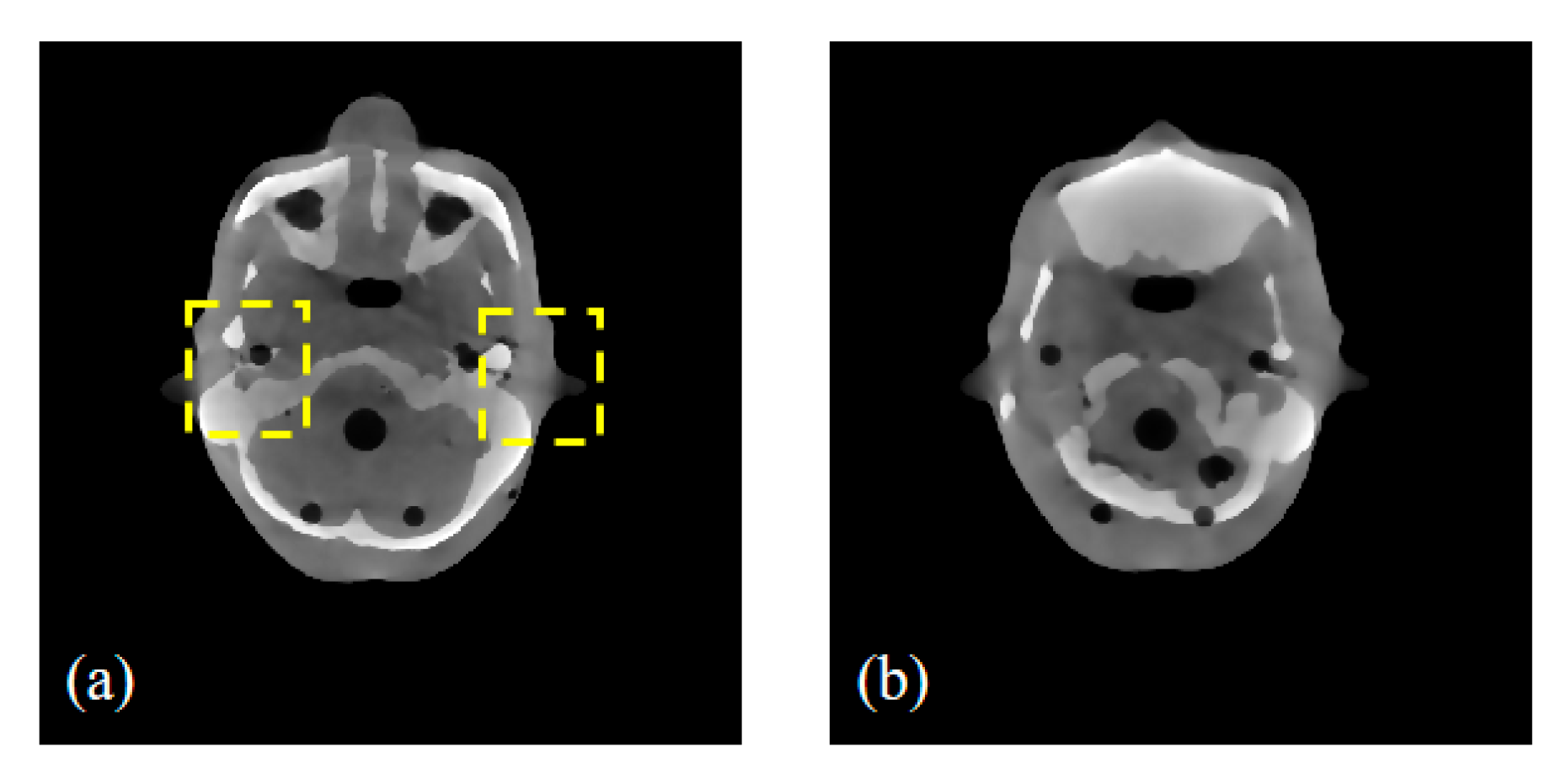
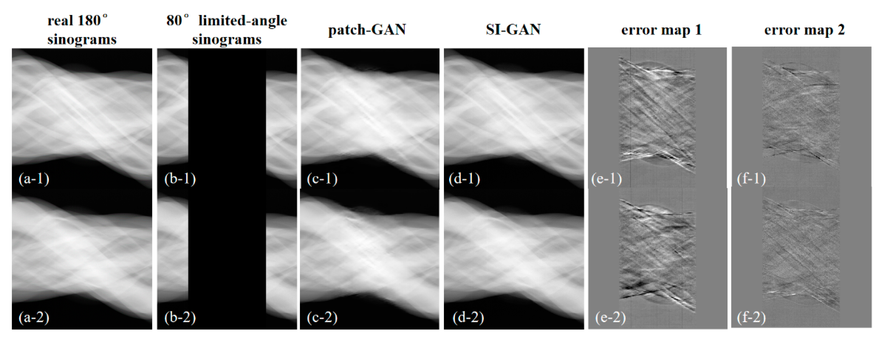
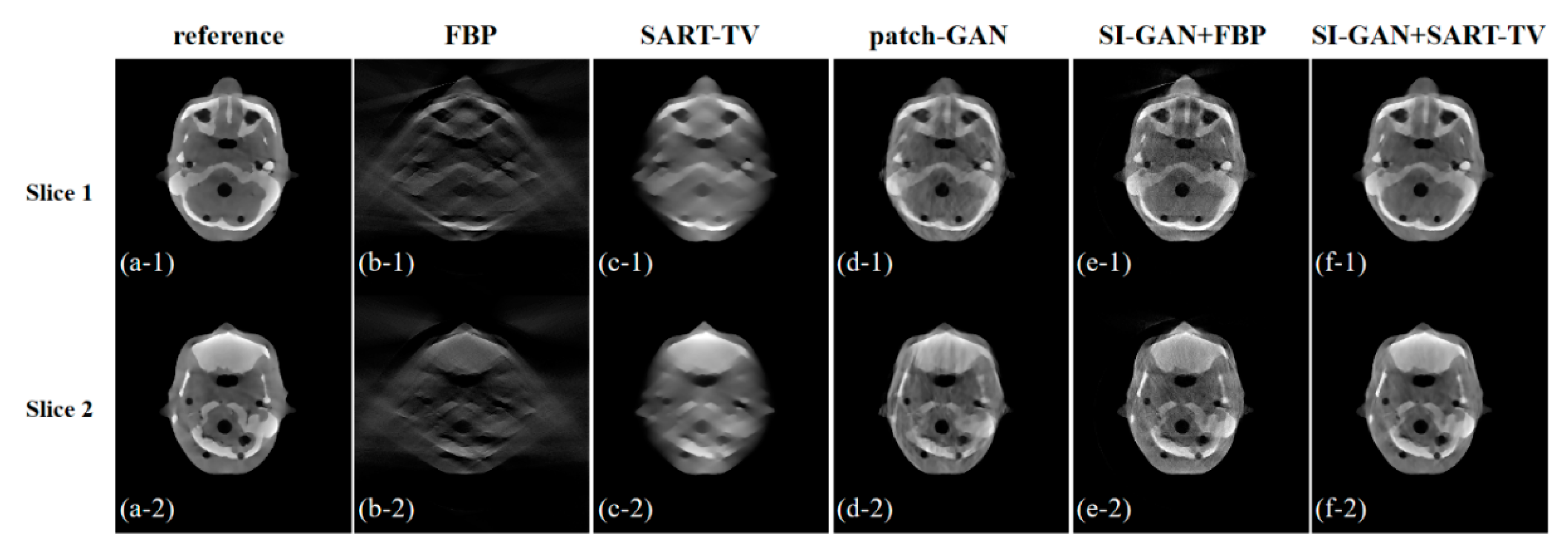
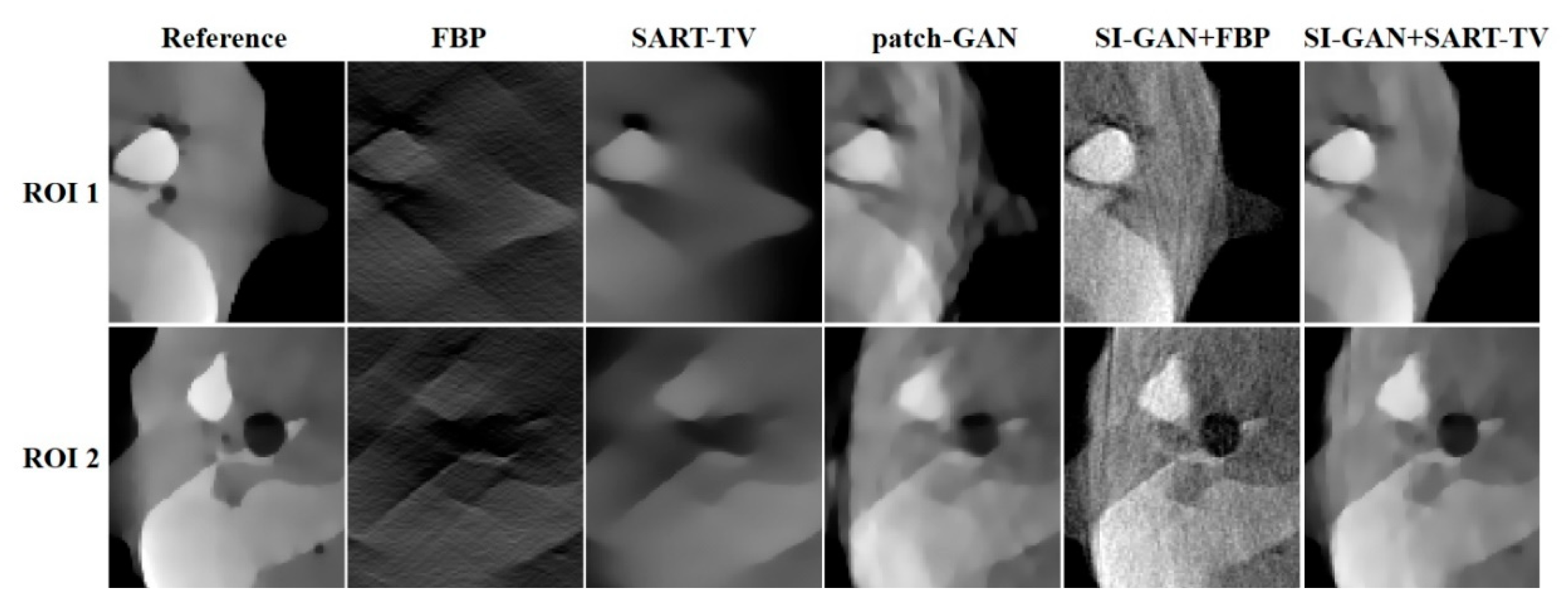
4.3. Real Data Study
5. Discussion and Conclusions
Author Contributions
Funding
Acknowledgments
Conflicts of Interest
References
- Zhang, Y.; Chan, H.B.; Wei, J.; Goodsitt, M.M.; Hadjiiski, L.M.; Ge, J.; Zhou, C. A comparative study of limited-angle cone-beam reconstruction methods for breast tomosynthesis. Med. Phys. 2006, 33, 3781–3795. [Google Scholar] [CrossRef] [PubMed]
- Inouye, T. Image reconstruction with limited angle projection. IEEE Trans. Nucl. Sci. 1979, 26, 2665–2669. [Google Scholar] [CrossRef]
- Tam, K.C.; Perezmendez, V. Tomographical imaging with limited-angle input. J. Opt. Soc. Am. 2013, 71, 582–592. [Google Scholar] [CrossRef]
- Andersen, A.H. Algebraic reconstruction in CT from limited views. IEEE Trans. Med. Imaging 1989, 8, 50–55. [Google Scholar] [CrossRef] [PubMed]
- Smith, B.D. Image Reconstruction from Cone-Beam Projections: Necessary and Sufficient Conditions and Reconstruction Methods. IEEE Trans. Med. Imaging 1985, 4, 14–25. [Google Scholar] [CrossRef] [PubMed]
- Tuy, H.K. An Inversion Formula for Cone-Beam Reconstruction. Siam J. Appl. Math. 1983, 43, 546–552. [Google Scholar] [CrossRef]
- Natterer, F. The Mathematics of Computerized Tomography; Springer: Wiesbaden, Germany, 1986. [Google Scholar]
- Katsevich, A. Theoretically Exact Filtered Backprojection-Type Inversion Algorithm for Spiral CT. Siam J. Appl. Math. 2002, 62, 2012–2026. [Google Scholar] [CrossRef]
- Gao, H.; Zhang, L.; Chen, Z.; Xing, Y.; Qi, Z. Direct filtered-backprojection-type reconstruction from a straight-line trajectory. Opt. Eng. 2007, 46, 057003. [Google Scholar] [CrossRef]
- Yu, H.; Wang, G. Compressed sensing based interior tomography. Phys. Med. Biol. 2009, 54, 2791–2805. [Google Scholar] [CrossRef]
- Zhang, H.M.; Wang, L.Y.; Yan, B.; Lei, L.; Xi, X.Q.; Lu, L.Z. Image reconstruction based on total-variation minimization and alternating direction method in linear scan computed tomography. Chin. Phys. B 2013, 22, 582–589. [Google Scholar] [CrossRef]
- Han, X.; Bian, J.; Ritman, E.L.; Sidky, E.Y.; Pan, X. Optimization-based reconstruction of sparse images from few-view projections. Phys. Med. Biol. 2012, 57, 5245–5273. [Google Scholar] [CrossRef] [PubMed]
- Rantala, M.; Vanska, S.; Jarvenpaa, S.; Kalke, M.; Lassas, M.; Moberg, J.; Siltanen, S. Wavelet-based reconstruction for limited-angle X-ray tomography. IEEE Trans. Med. Imaging 2006, 25, 210. [Google Scholar] [CrossRef] [PubMed]
- Sidky, E.Y.; Pan, X. Image reconstruction in circular cone-beam computed tomography by constrained, total-variation minimization. Phys. Med. Biol. 2008, 53, 4777–4807. [Google Scholar] [CrossRef] [PubMed]
- Sidky, E.Y.; Kao, C.M.; Pan, X. Accurate image reconstruction from few-views and limited-angle data in divergent-beam CT. J. X-ray Sci. Technol. 2009, 14, 119–139. [Google Scholar]
- Ritschl, L.; Bergner, F.; Fleischmann, C.; Kachelriess, M. Improved total variation-based CT image reconstruction applied to clinical data. Phys. Med. Biol. 2011, 56, 1545–1561. [Google Scholar] [CrossRef] [PubMed]
- Chen, G.J.; Leng, S. Prior image constrained compressed sensing (PICCS): A method to accurately reconstruct dynamic CT images from highly undersampled projection data sets. Proc. SPIE 2008, 6856, 685618. [Google Scholar] [CrossRef]
- Cai, A.; Wang, L.; Zhang, H.; Yan, B.; Li, L.; Xi, X.; Li, J. Edge guided image reconstruction in linear scan CT by weighted alternating direction TV minimization. J. X-ray Sci. Technol. 2014, 22, 335–349. [Google Scholar]
- Zhang, W.; Zhang, H.; Li, L.; Wang, L.; Cai, A.; Li, Z.; Yan, B. A promising limited angular computed tomography reconstruction via segmentation based regional enhancement and total variation minimization. Rev. Sci. Instrum. 2016, 87, 083104. [Google Scholar] [CrossRef]
- Natterer, F.; Wubbeling, F.; Wang, G. Mathematical Methods in Image Reconstruction. Med. Phys. 2002, 29, 107–108. [Google Scholar] [CrossRef]
- Yang, Y.; Sun, J.; Li, H.; Xu, Z. ADMM-Net: A Deep Learning Approach for Compressive Sensing MRI. arXiv 2017, arXiv:1705.06869. [Google Scholar]
- Hinton, G.E.; Salakhutdinov, R.R. Supporting Online Material for “Reducing the Dimensionality of Data with Neural Networks”. Methods 2006, 313, 504–507. [Google Scholar]
- LeCun, Y.; Bengio, Y.; Hinton, G. Deep learning. Nature 2015, 521, 436–444. [Google Scholar] [CrossRef] [PubMed]
- Wang, G. A Perspective on Deep Imaging. IEEE Access 2017, 4, 8914–8924. [Google Scholar] [CrossRef]
- Chen, H.; Zhang, Y.; Kalra, M.K.; Lin, F.; Chen, Y.; Liao, P.; Zhou, J.; Wang, G. Low-Dose CT with a Residual Encoder-Decoder Convolutional Neural Network (RED-CNN). IEEE Trans. Med Imaging 2017, 36, 2524–2535. [Google Scholar] [CrossRef] [PubMed]
- Wu, D.; Kim, K.; Dong, B.; Li, Q. End-to-End Abnormality Detection in Medical Imaging. arXiv 2018, arXiv:1711.02074. [Google Scholar]
- Lee, H.; Lee, J.; Cho, S. View-Interpolation of Sparsely Sampled Sinogram Using Convolutional Neural Network. In Medical Imaging 2017: Image Processing; Society of Photo-Optical Instrumentation Engineers: Bellingham, WA, USA, 2017; p. 1013328. [Google Scholar]
- Zhang, H.; Li, L.; Qiao, K.; Wang, L.; Yan, B.; Li, L.; Hu, G. Image Prediction for Limited-angle Tomography via Deep Learning with Convolutional Neural Network. arXiv 2016, arXiv:1607.08707. [Google Scholar]
- Gu, J.; Ye, J.C. Multi-Scale Wavelet Domain Residual Learning for Limited-Angle CT Reconstruction. arXiv 2017, arXiv:1703.01382. [Google Scholar]
- Tovey, R.; Benning, M.; Brune, C.; Lagerwerf, M.J.; Collins, S.M.; Leary, R.K.; Midgley, P.A.; Schoenlieb, C.B. Directional Sinogram Inpainting for Limited Angle Tomography. arXiv 2018, arXiv:1804.09991. [Google Scholar] [CrossRef]
- Han, Y.; Kang, J.; Ye, J.C. Deep Learning Reconstruction for 9-View Dual Energy CT Baggage Scanner. arXiv 2018, arXiv:1801.01258. [Google Scholar]
- Liang, K.; Xing, Y.; Yang, H.; Kang, K. Improve angular resolution for sparse-view CT with residual convolutional neural network. In Proceedings of the SPIE Medical Imaging Conference, Houston, TX, USA, 10–15 February 2018. [Google Scholar]
- Liang, K.; Yang, H.; Xing, Y. Comparision of projection domain, image domain, and comprehensive deep learning for sparse-view X-ray CT image reconstruction. arXiv 2018, arXiv:1804.04289. [Google Scholar]
- Isola, P.; Zhu, J.Y.; Zhou, T.; Efros, A.A. Image-to-Image Translation with Conditional Adversarial Networks. In Proceedings of the CVPR 2017, Honolulu, HI, USA, 21–26 July 2017; pp. 5967–5976. [Google Scholar]
- Yi, Z.; Zhang, H.; Gong, P.T.M.; Yi, Z.; Zhang, H.; Gong, P.T.M.; Yi, Z.; Zhang, H.; Gong, P.T.M. DualGAN: Unsupervised Dual Learning for Image-to-Image Translation. In Proceedings of the ICCV 2017, Venice, Italy, 22–29 Octorber 2017; pp. 2868–2876. [Google Scholar]
- Xu, J.; Sun, X.; Ren, X.; Lin, J.; Wei, B.; Li, W. DP-GAN: Diversity-Promoting Generative Adversarial Network for Generating Informative and Diversified Text. arXiv 2018, arXiv:1802.01345. [Google Scholar]
- Zhu, J.Y.; Park, T.; Isola, P.; Efros, A.A. Unpaired Image-to-Image Translation Using Cycle-Consistent Adversarial Networks. In Proceedings of the IEEE International Conference on Computer Vision, Venice, Italy, 22–29 Octorber 2017. [Google Scholar]
- Jin, S.C.; Hsieh, C.J.; Chen, J.C.; Tu, S.H.; Kuo, C.W. Development of Limited-Angle Iterative Reconstruction Algorithms with Context Encoder-Based Sinogram Completion for Micro-CT Applications. Sensors 2018, 18, 4458. [Google Scholar] [CrossRef] [PubMed]
- Li, Z.; Zhang, W.; Wang, L.; Cai, A.; Li, L. A Sinogram Inpainting Method based on Generative Adversarial Network for Limited-angle Computed Tomography. In Proceedings of the SPIE 11072, 15th International Meeting on Fully Three-Dimensional Image Reconstruction in Radiology and Nuclear Medicine, Philadelphia, PA, USA, 2–6 June 2019. [Google Scholar]
- Zhao, J.; Chen, Z.; Zhang, L.; Jin, X. Unsupervised Learnable Sinogram Inpainting Network (SIN) for Limited Angle CT reconstruction. arXiv 2018, arXiv:1811.03911. [Google Scholar]
- Radford, A.; Metz, L.; Chintala, S. Unsupervised Representation Learning with Deep Convolutional Generative Adversarial Networks. arXiv 2015, arXiv:1511.06434. [Google Scholar]
- Mirza, M.; Osindero, S. Conditional Generative Adversarial Nets. arXiv 2014, arXiv:1411.1784. [Google Scholar]
- Dar, S.U.H.; Yurt, M.; Karacan, L.; Erdem, A.; Erdem, E.; Çukur, T. Image Synthesis in Multi-Contrast MRI with Conditional Generative Adversarial Networks. IEEE Trans. Med Imaging 2018. [Google Scholar] [CrossRef]
- Ganguli, S.; Garzon, P.; Glaser, N. GeoGAN: A Conditional GAN with Reconstruction and Style Loss to Generate Standard Layer of Maps from Satellite Images. arXiv 2019, arXiv:1902.05611. [Google Scholar]
- Qiao, T.; Zhang, W.; Zhang, M.; Ma, Z.; Xu, D. Ancient Painting to Natural Image: A New Solution for Painting Processing. arXiv 2019, arXiv:1901.00224. [Google Scholar]
- Aarle, W.V.; Palenstijn, W.J.; Beenhouwer, J.D.; Altantzis, T.; Bals, S.; Batenburg, K.J.; Sijbers, J. The ASTRA Toolbox: A platform for advanced algorithm development in electron tomography. Ultramicroscopy 2015, 157, 35–47. [Google Scholar] [CrossRef]
- Ronneberger, O.; Fischer, P.; Brox, T. U-Net: Convolutional Networks for Biomedical Image Segmentation. In Proceedings of the International Conference on Medical Image Computing & Computer-assisted Intervention, Munich, Germany, 5–9 October 2015. [Google Scholar]
- Luo, W.; Li, Y.; Urtasun, R.; Zemel, R. Understanding the Effective Receptive Field in Deep Convolutional Neural Networks. arXiv 2017, arXiv:1701.04128. [Google Scholar]
- Li, C.; Wand, M. Precomputed Real-Time Texture Synthesis with Markovian Generative Adversarial Networks. In Proceedings of the ECCV, Amsterdam, The Netherlands, 11–14 October 2016. [Google Scholar]
- Li, C.; Wand, M. Combining Markov Random Fields and Convolutional Neural Networks for Image Synthesis. In Proceedings of the CVPR, Las Vegas, NV, USA, 27–30 June 2016. [Google Scholar]
- Siddon, R.L. Fast calculation of the exact radiological path for a three-dimensional CT array. Med. Phys. 1985, 12, 252. [Google Scholar] [CrossRef] [PubMed]
- Elaiyaraja, G.; Kumaratharan, N.; Rao, T.C.S. Fast and Efficient Filter Using Wavelet Threshold for Removal of Gaussian Noise from MRI/CT Scanned Medical Images/Color Video Sequence. IETE J. Res. 2019, 1–13. [Google Scholar] [CrossRef]
- ICRU. Phantoms and Computational Models in Therapy, Diagnosis and Protcction; Report No. 48; ICRU: Bethesda, MD, USA, 1992. [Google Scholar]
- Zhou, W.; Alan Conrad, B.; Hamid Rahim, S.; Simoncelli, E.P. Image quality assessment: From error visibility to structural similarity. IEEE Trans. Image Process. 2004, 13, 600–612. [Google Scholar]


| Procedure: Establishment of the training dataset |
|
| On the basis of the above procedure, 5000 pairs of input and label sinograms with size of 512 × 512 were prepared. |
| Parameters | For SI-GAN Training | For SI-GAN Testing |
|---|---|---|
| Detector elements | 512 | 512 |
| Detector bin size (mm) | 0.831 | 0.831 |
| Distance of source to object (mm) | 483.41 | 462.66 |
| Distance of source to detector (mm) | 796.49 | 870.96 |
| Tube voltage (kVp) | 120 | 120 |
| Tube current (A) | 209 | 210 |
| Number of projections | 512 | 512 |
| Scanning range (°) | 180 | 180 |
| Reconstruction size | 512 × 512 | 512 × 512 |
| avg. PSNR | avg. RMSE | avg. NMAD | avg. SSIM | |
|---|---|---|---|---|
| FBP | 17.234 | 0.0553 | 1.5684 | 0.2631 |
| SART-TV | 18.792 | 0.0317 | 0.6512 | 0.7479 |
| patch-GAN | 28.369 | 0.0131 | 0.1828 | 0.9433 |
| SI-GAN () + FBP | 27.230 | 0.0164 | 0.3493 | 0.8513 |
| SI-GAN () + SART-TV | 28.122 | 0.0139 | 0.1933 | 0.9466 |
| SI-GAN + FBP | 29.209 | 0.0114 | 0.2689 | 0.8657 |
| SI-GAN + SART-TV | 31.052 | 0.0093 | 0.1264 | 0.9648 |
| avg. PSNR | avg. RMSE | avg. NMAD | avg. SSIM | |
|---|---|---|---|---|
| SART-TV | 15.117 | 0.0407 | 0.9306 | 0.6149 |
| patch-GAN | 27.460 | 0.0141 | 0.2033 | 0.9327 |
| SI-GAN + SART-TV | 29.820 | 0.0097 | 0.1467 | 0.9588 |
| PSNR | RMSE | NMAD | SSIM | ||
|---|---|---|---|---|---|
| Slice 1 | FBP | 13.6388 | 2.52 × 10⁻³ | 0.9820 | 0.9564 |
| SART-TV | 21.9823 | 1.02 × 10⁻³ | 0.2843 | 0.9939 | |
| patch-GAN | 29.6305 | 4.04 × 10⁻⁴ | 0.1002 | 0.9983 | |
| SI-GAN + FBP | 24.4512 | 9.55 × 10⁻⁴ | 0.3874 | 0.9929 | |
| SI-GAN + SART-TV | 35.3856 | 2.25 × 10⁻⁴ | 0.0504 | 0.9989 | |
| Slice 2 | FBP | 11.4794 | 2.44 × 10⁻³ | 0.9954 | 0.9589 |
| SART-TV | 23.5963 | 8.71 × 10⁻⁴ | 0.2603 | 0.9953 | |
| patch-GAN | 29.8019 | 4.01 × 10⁻⁴ | 0.1162 | 0.9982 | |
| SI-GAN + FBP | 24.4064 | 9.07 × 10⁻⁴ | 0.3882 | 0.9935 | |
| SI-GAN + SART-TV | 35.1920 | 2.41 × 10⁻⁴ | 0.0714 | 0.9987 |
| avg. RMSE | avg. NMAD | ||
|---|---|---|---|
| patch-GAN | Test one (90°) | 0.01094 | 0.02636 |
| Test two (60°) | 0.01227 | 0.03570 | |
| SI-GAN | Test one (90°) | 0.00547 | 0.01297 |
| Test two (60°) | 0.00601 | 0.01790 |
© 2019 by the authors. Licensee MDPI, Basel, Switzerland. This article is an open access article distributed under the terms and conditions of the Creative Commons Attribution (CC BY) license (http://creativecommons.org/licenses/by/4.0/).
Share and Cite
Li, Z.; Cai, A.; Wang, L.; Zhang, W.; Tang, C.; Li, L.; Liang, N.; Yan, B. Promising Generative Adversarial Network Based Sinogram Inpainting Method for Ultra-Limited-Angle Computed Tomography Imaging. Sensors 2019, 19, 3941. https://doi.org/10.3390/s19183941
Li Z, Cai A, Wang L, Zhang W, Tang C, Li L, Liang N, Yan B. Promising Generative Adversarial Network Based Sinogram Inpainting Method for Ultra-Limited-Angle Computed Tomography Imaging. Sensors. 2019; 19(18):3941. https://doi.org/10.3390/s19183941
Chicago/Turabian StyleLi, Ziheng, Ailong Cai, Linyuan Wang, Wenkun Zhang, Chao Tang, Lei Li, Ningning Liang, and Bin Yan. 2019. "Promising Generative Adversarial Network Based Sinogram Inpainting Method for Ultra-Limited-Angle Computed Tomography Imaging" Sensors 19, no. 18: 3941. https://doi.org/10.3390/s19183941
APA StyleLi, Z., Cai, A., Wang, L., Zhang, W., Tang, C., Li, L., Liang, N., & Yan, B. (2019). Promising Generative Adversarial Network Based Sinogram Inpainting Method for Ultra-Limited-Angle Computed Tomography Imaging. Sensors, 19(18), 3941. https://doi.org/10.3390/s19183941