AI-Based Early Change Detection in Smart Living Environments


Abstract
:1. Introduction
2. State-of-the-Art and Related Work
3. Materials and Methods
- [St] Starting time of activity. This is a change in the starting time of an activity, e.g., having breakfast at 9 AM instead of 7 AM as usual.
- [Du] Duration of activity. This change refers to the duration of an activity, e.g., resting for 3 hours in the afternoon, instead of 1 hour as usual.
- [Di] Disappearing of activity. In this case, after the change, one activity is no more performed by the user, e.g., having physical exercises in the afternoon.
- [Sw] Swap of two activities. After the change, two activities are per-formed in reverse order, e.g., resting and then housekeeping instead of housekeeping and resting.
- [Lo] Location of activity. One activity usually performed in a home location (e.g., having breakfast in the kitchen), after the change is performed in a different location (e.g., having breakfast in bed).
- [Hr] Heartrate during activity. This is a change in heartrate during an activity, e.g., changing from a low to a high heartrate during the resting activity in the afternoon.
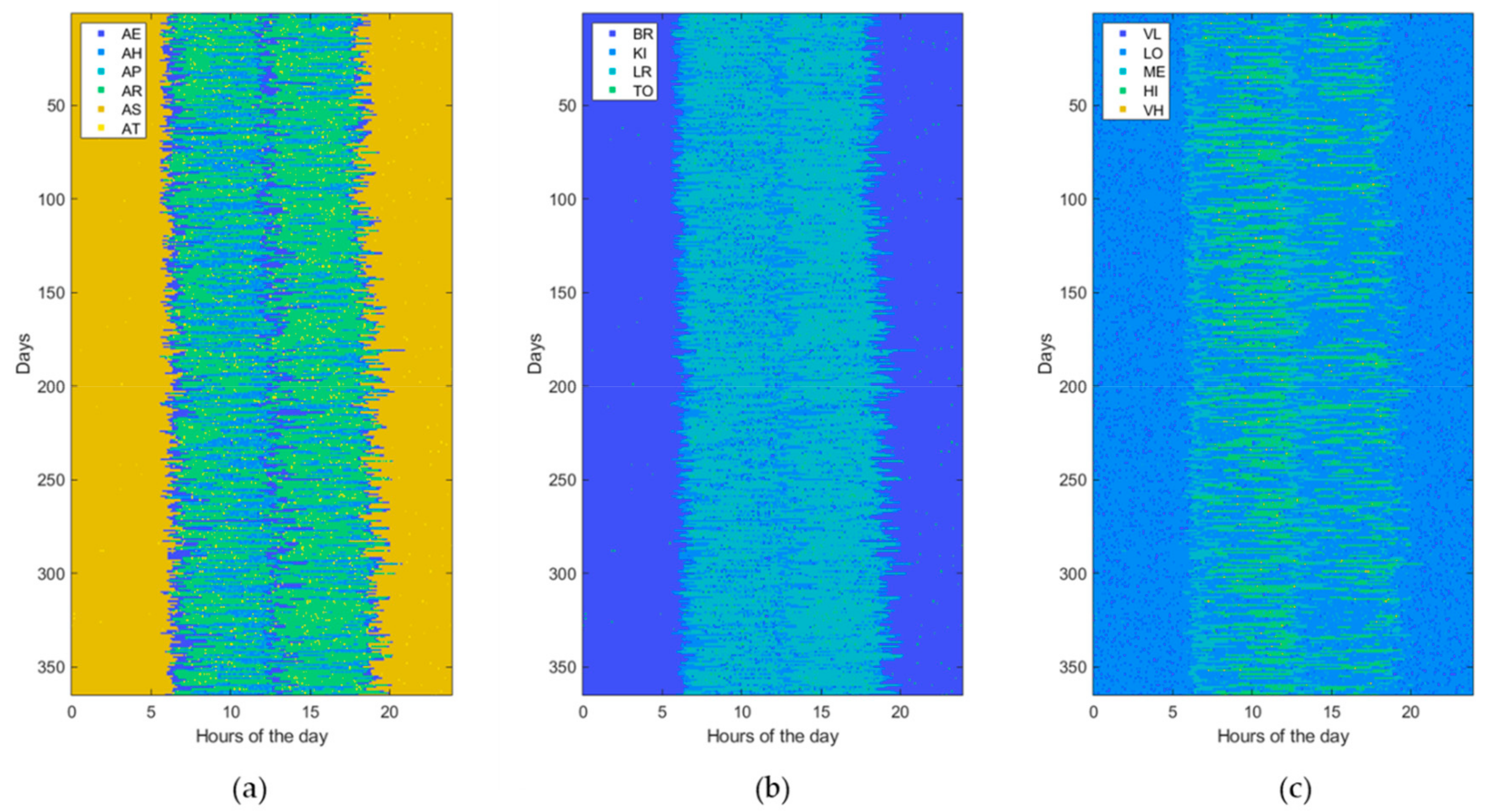
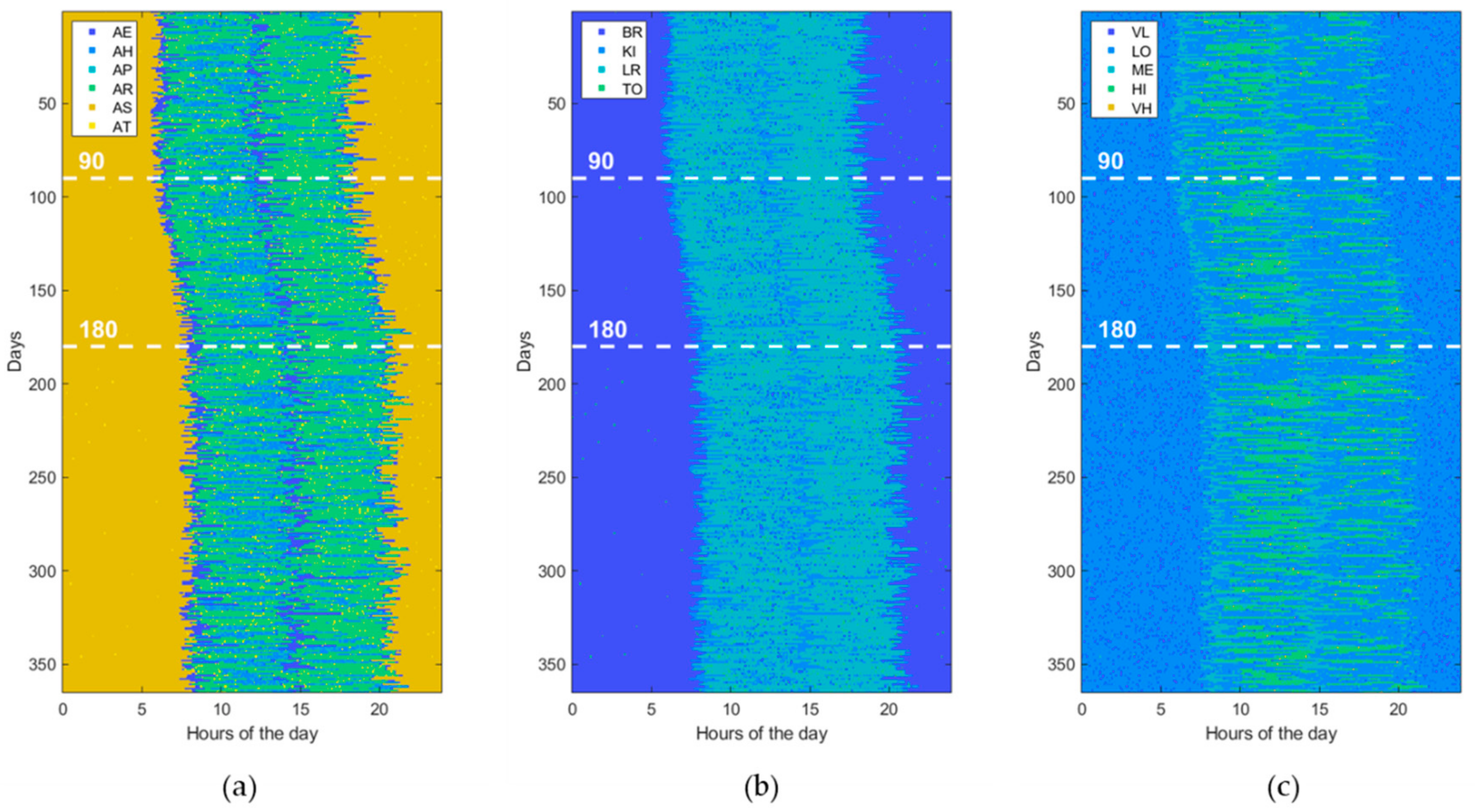
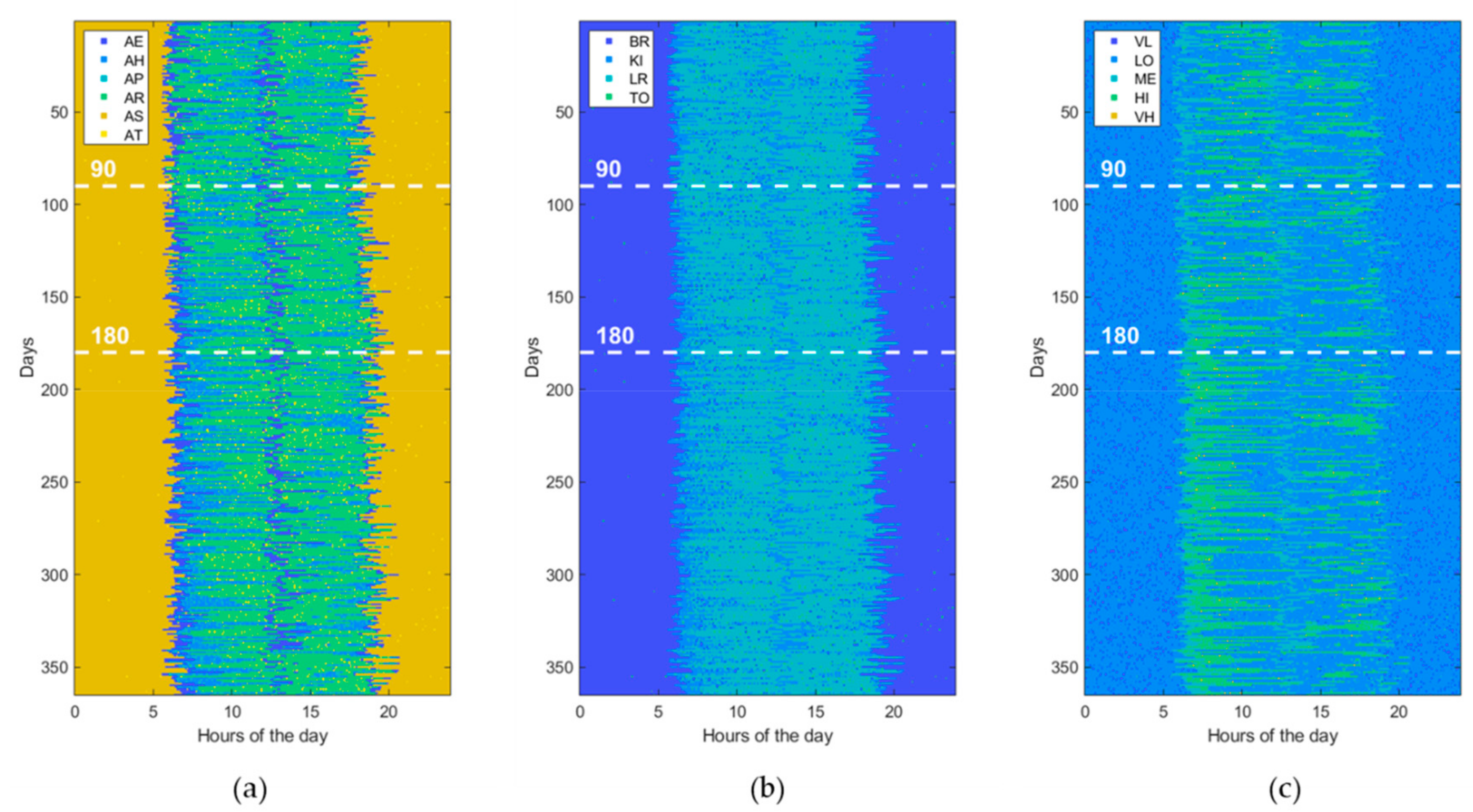
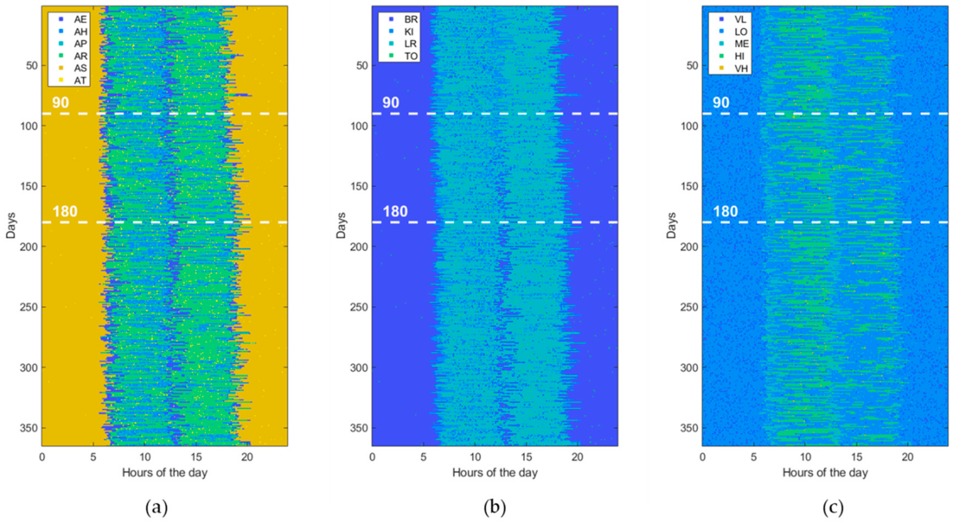
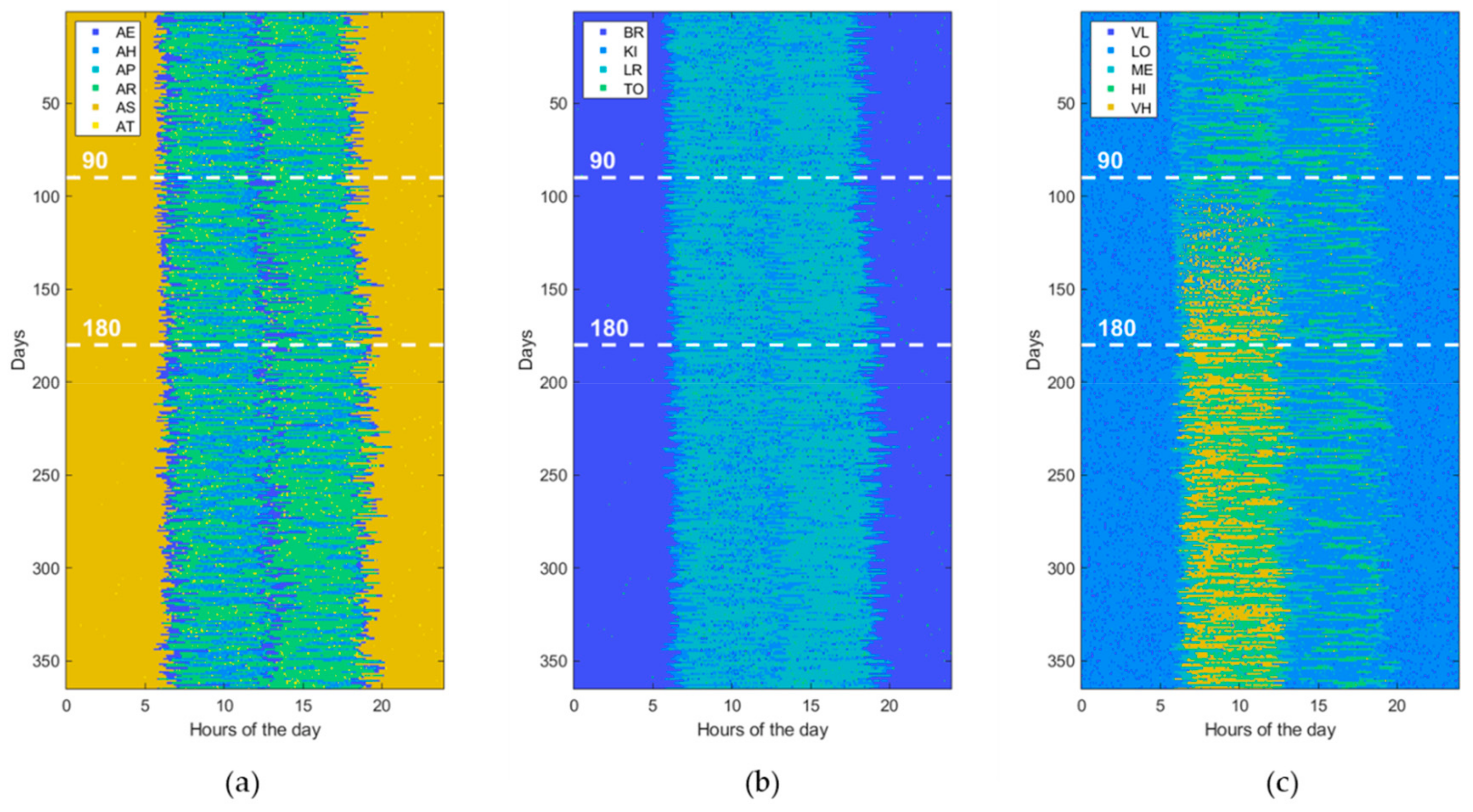
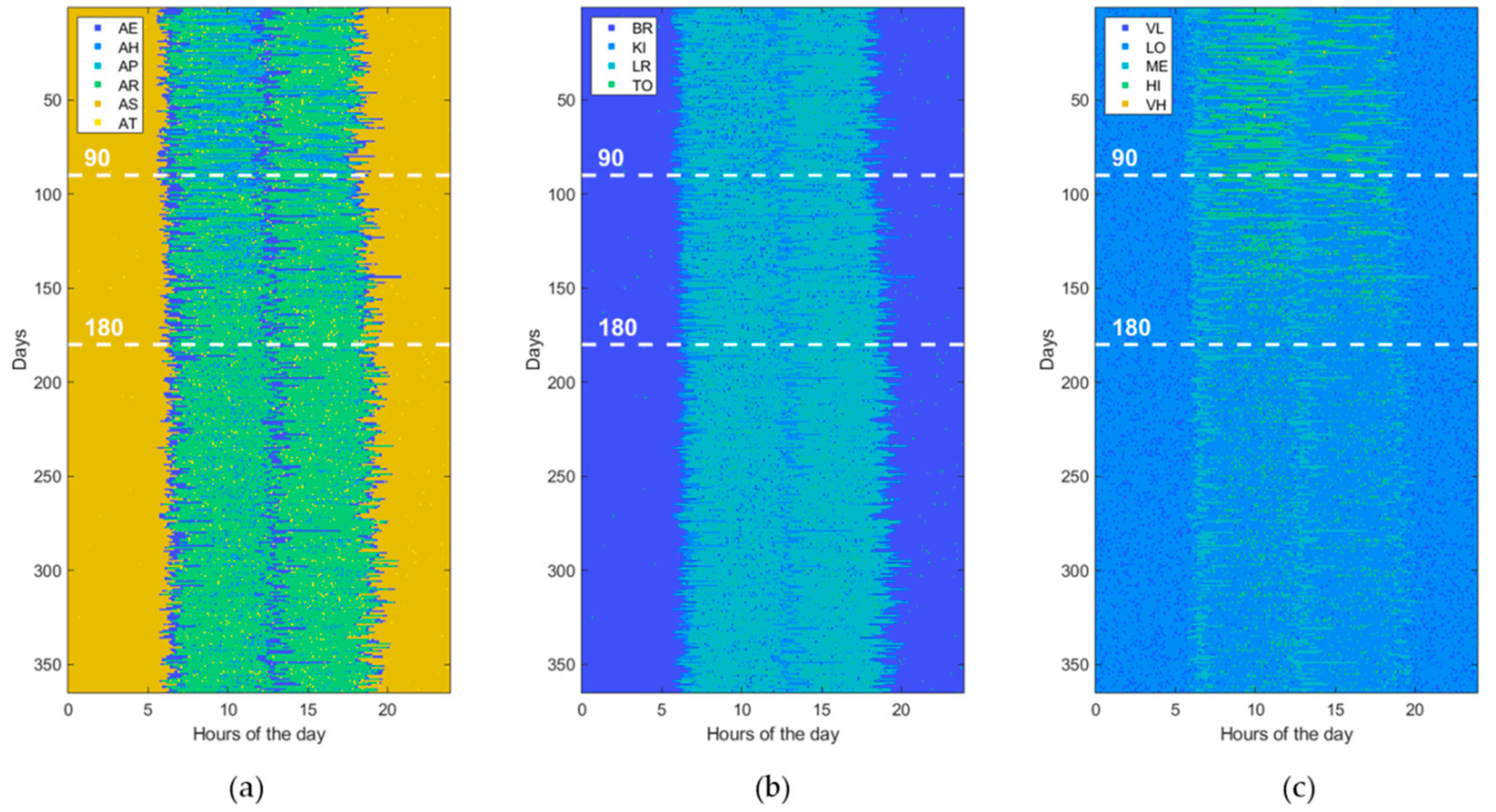
3.1. Data Generation
3.2. Learning Techniques for Abnormal Behavior Detection
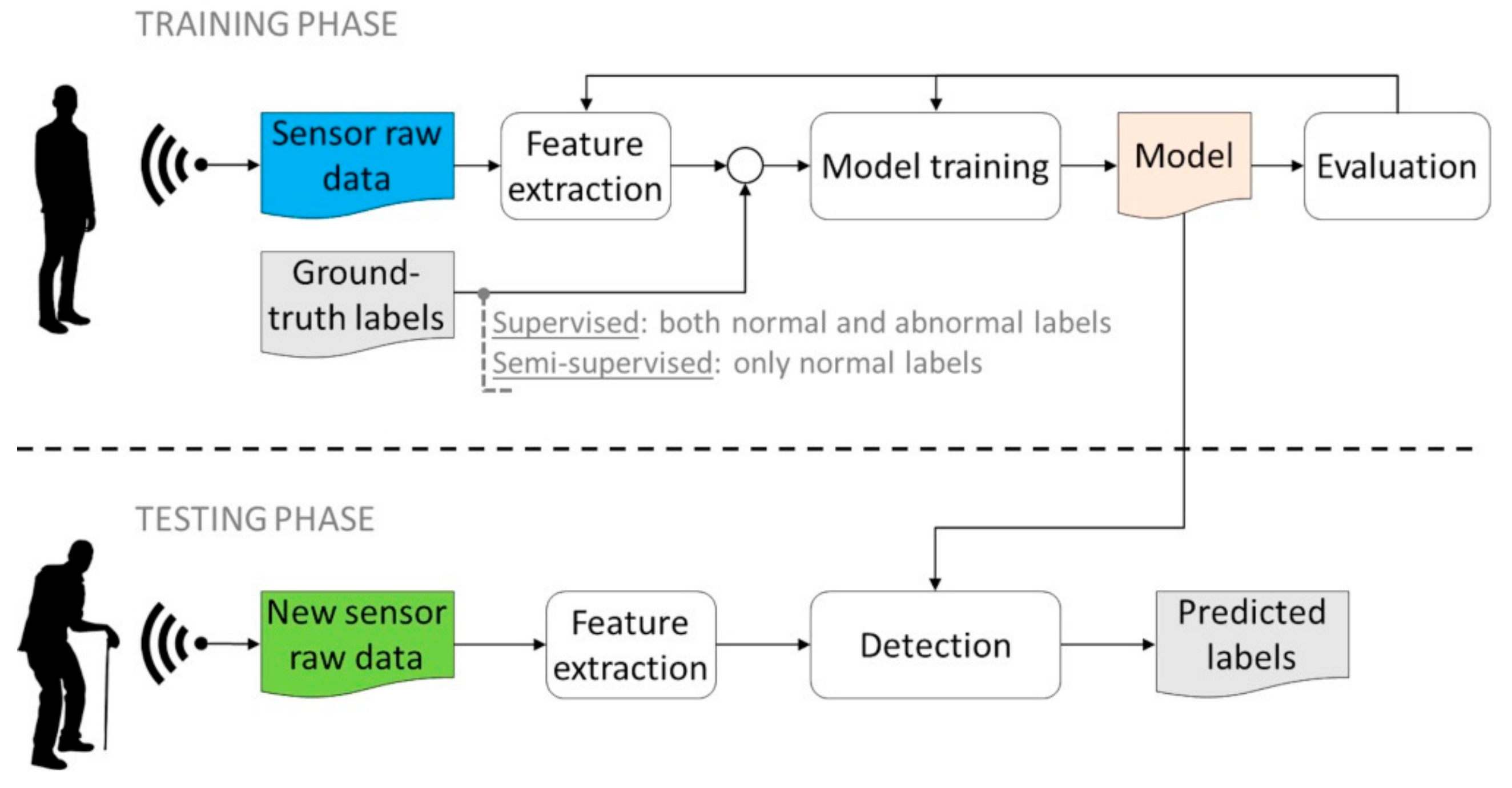
3.2.1. Supervised Detection
3.2.2. Semi-Supervised Detection
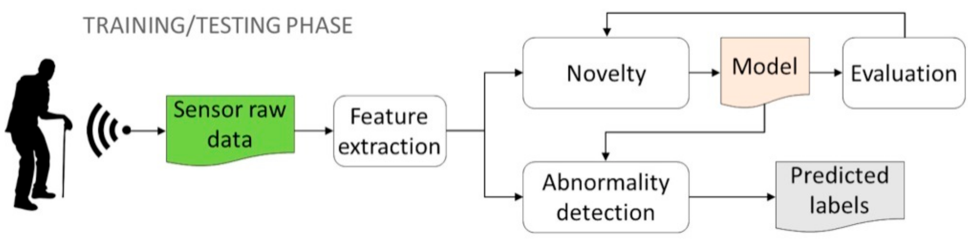
3.2.3. Unsupervised Detection
3.3. Experimental Setting
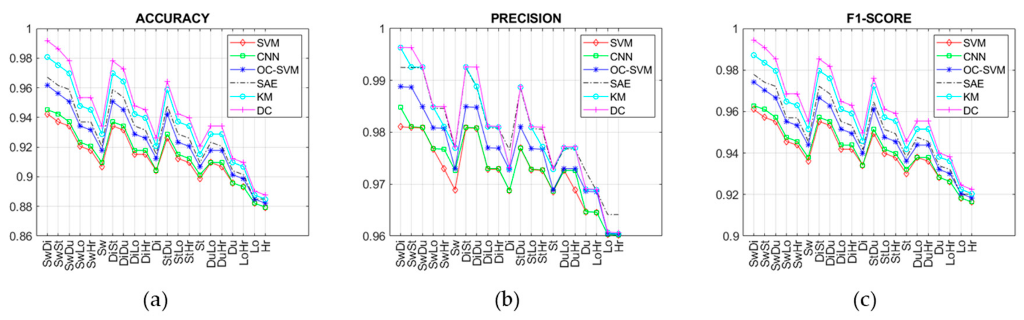
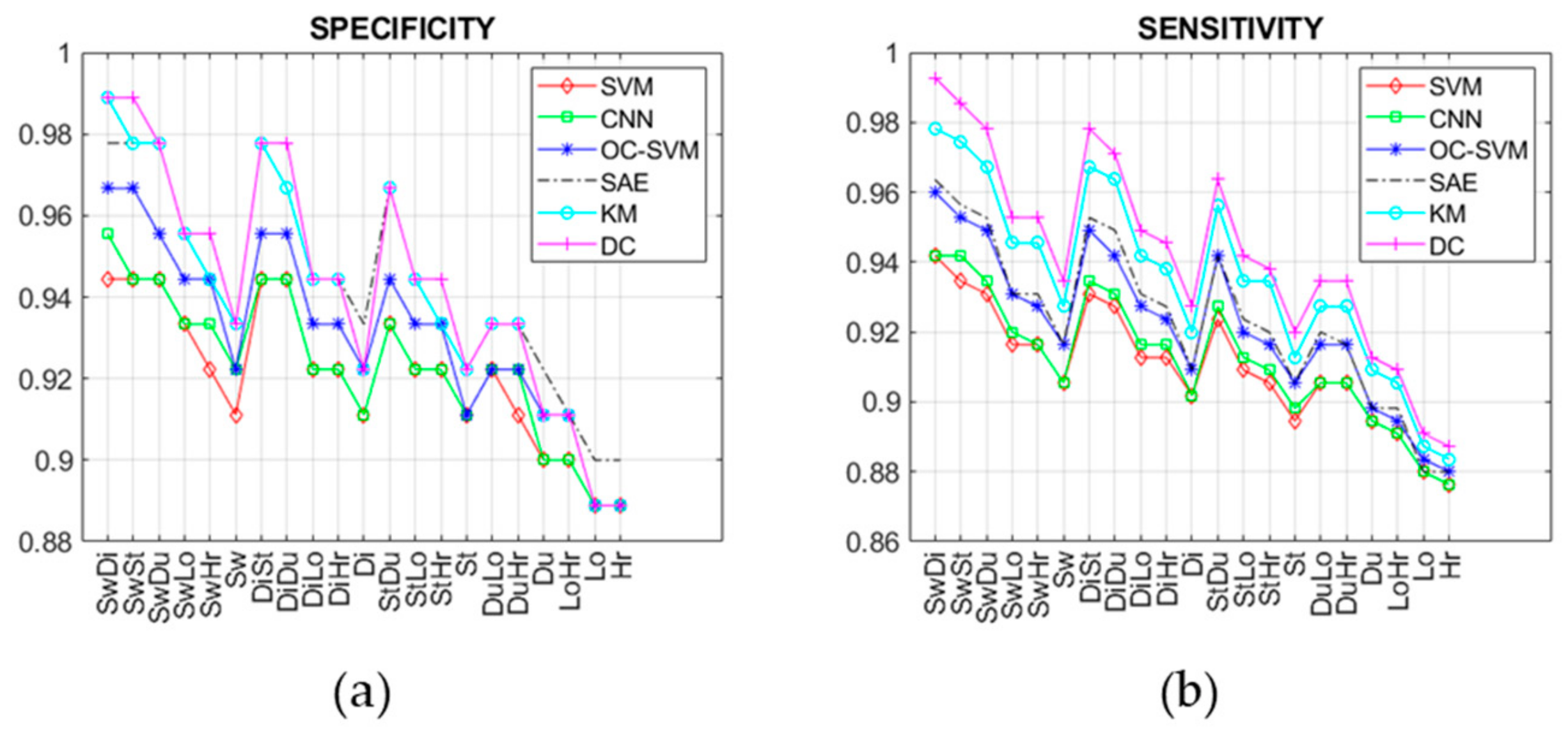
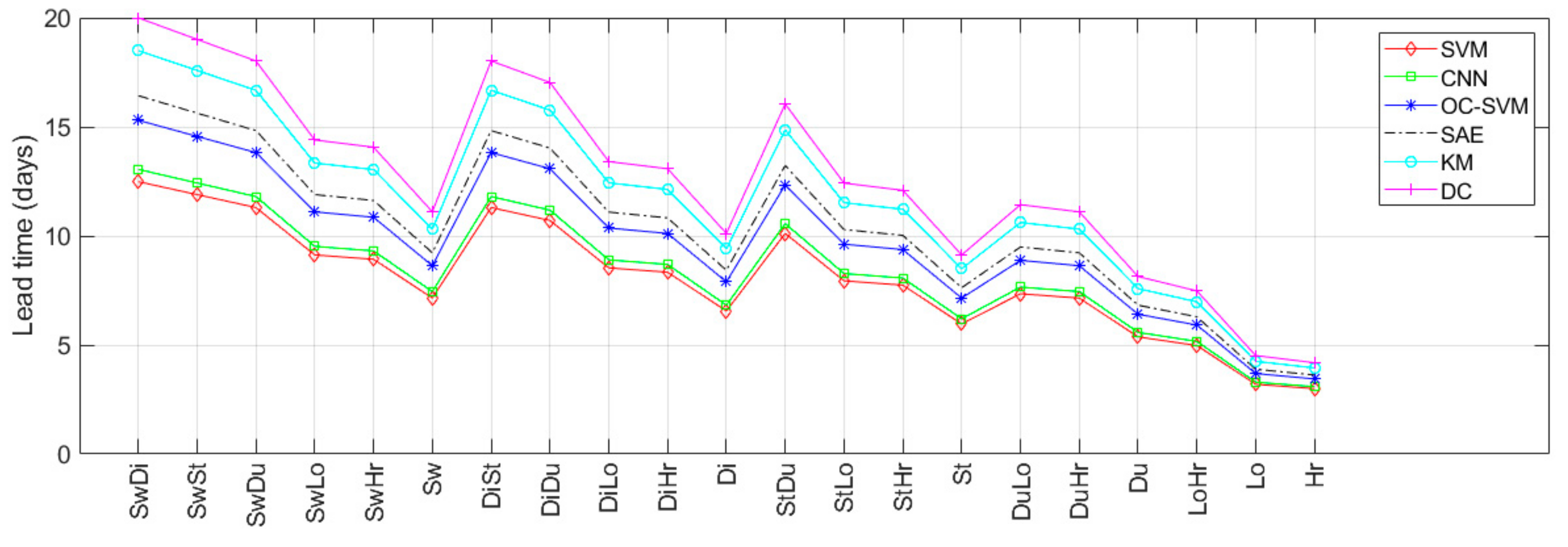
4. Results
5. Discussion
6. Conclusions
Author Contributions
Funding
Conflicts of Interest
References
- Gokalp, H.; Clarke, M. Monitoring activities of daily living of the elderly and the potential for its use in telecare and telehealth: A review. Telemed. E-Health 2013, 19, 910–923. [Google Scholar] [CrossRef] [PubMed]
- Sharma, R.; Nah, F.; Sharma, K.; Katta, T.; Pang, N.; Yong, A. Smart living for elderly: De-sign and human-computer interaction considerations. Lect. Notes Comput. Sci. 2016, 9755, 112–122. [Google Scholar]
- Parisa, R.; Mihailidis, A. A survey on ambient-assisted living tools for older adults. IEEE J. Biomed. Health Inform. 2013, 17, 579–590. [Google Scholar]
- Vimarlund, V.; Wass, S. Big data, smart homes and ambient assisted living. Yearb. Med. Inform. 2014, 9, 143–149. [Google Scholar]
- Mabrouk, A.B.; Zagrouba, E. Abnormal behavior recognition for intelligent video surveil-lance systems: A review. Expert Syst. Appl. 2018, 91, 480–491. [Google Scholar] [CrossRef]
- Bakar, U.; Ghayvat, H.; Hasanm, S.F.; Mukhopadhyay, S.C. Activity and anomaly detection in smart home: A survey. Next Gener. Sens. Syst. 2015, 16, 191–220. [Google Scholar]
- Diraco, G.; Leone, A.; Siciliano, P.; Grassi, M.; Malcovati, P. A Multi-Sensor System for Fall Detection in Ambient Assisted Living Contexts. IEEE Sens. 2012, 213–219. [Google Scholar] [CrossRef]
- Taraldsen, K.; Chastin, S.F.M.; Riphagen, I.I.; Vereijken, B.; Helbostad, J.L. Physical activity monitoring by use of accelerometer-based body-worn sensors in older adults: A systematic literature review of current knowledge and applications. Maturitas 2012, 71, 13–19. [Google Scholar] [CrossRef]
- Min, C.; Kang, S.; Yoo, C.; Cha, J.; Choi, S.; Oh, Y.; Song, J. Exploring current practices for battery use and management of smartwatches. In Proceedings of the ISWC ′15 Proceedings of the 2015 ACM International Symposium on Wearable Computers, Osaka, Japan, 7–11 September 2015. [Google Scholar]
- Stara, V.; Zancanaro, M.; Di Rosa, M.; Rossi, L.; Pinnelli, S. Understanding the Interest Toward Smart Home Technology: The Role of Utilitaristic Perspective. In ForItAAL; Springer: Berlin, Germany, 2018. [Google Scholar]
- Droghini, D.; Ferretti, D.; Principi, E.; Squartini, S.; Piazza, F. A Combined One-Class SVM and Template-Matching Approach for User-Aided Human Fall Detection by Means of Floor Acoustic Features. Comput. Intell. Neurosci. 2017, 2017, 1–13. [Google Scholar] [CrossRef] [Green Version]
- Hussmann, S.; Ringbeck, T.; Hagebeuker, B. A performance review of 3D TOF vision systems in comparison to stereo vision systems. In Stereo Vision; InTech: Rijeka, Croatia, 2008. [Google Scholar]
- Diraco, G.; Leone, A.; Siciliano, P. Radar sensing technology for fall detection under near real-life conditions. In Proceedings of the IET Conference, London, UK, 24–25 October 2016. [Google Scholar]
- Lazaro, A.; Girbau, D.; Villarino, R. Analysis of vital signs monitoring using an IR-UWB radar. Prog. Electromagn. Res. 2010, 100, 265–284. [Google Scholar] [CrossRef]
- Diraco, G.; Leone, A.; Siciliano, P. A radar-based smart sensor for unobtrusive elderly monitoring in ambient assisted living applications. Biosensors 2017, 7, 55. [Google Scholar] [CrossRef] [PubMed]
- Caroppo, A.; Diraco, G.; Rescio, G.; Leone, A.; Siciliano, P. Heterogeneous sensor platform for circadian rhythm analysis. In Proceedings of the 2015 6th International Workshop on Advances in Sensors and Interfaces (IWASI), Gallipoli, Italy, 10 August 2015. [Google Scholar]
- Dong, H.; Evans, D. Data-fusion techniques and its application. In Proceedings of the Fourth International Conference on Fuzzy Systems and Knowledge Discovery (FSKD 2007), Haikou, China, 24–27 August 2007. [Google Scholar]
- Miao, Y.; Song, J. Abnormal Event Detection Based on SVM in Video Surveillance. In Proceedings of the IEEE Workshop on Advance Research and Technology in Industry Applications, Ottawa, ON, Canada, 29–30 September 2014. [Google Scholar]
- Forkan, A.R.M.; Khalil, I.; Tari, Z.; Foufou, S.; Bouras, A. A context-aware approach for long-term behavioural change detection and abnormality prediction in ambient assisted living. Pattern Recognit. 2015, 48, 628–641. [Google Scholar] [CrossRef]
- Krizhevsky, A.; Sutskever, I.; Hinton, G.E. Imagenet classification with deep convolutional neural networks. In Proceedings of the Advances in neural information processing systems, Lake Tahoe, NV, USA, 3–6 December 2012. [Google Scholar]
- Hejazi, M.; Singh, Y.P. One-class support vector machines approach to anomaly detection. Appl. Artif. Intell. 2013, 27, 351–366. [Google Scholar] [CrossRef]
- Krizhevsky, A.; Hinton, G.E. Using very deep autoencoders for content-based image retrieval. In Proceedings of the 19th European Symposium on Artificial Neural Networks, Bruges, Belgium, 27–29 April 2011. [Google Scholar]
- Otte, F.J.P.; Saurer, R.B.; Stork, W. Unsupervised Learning in Ambient Assisted Living for Pattern and Anomaly Detection: A Survey. In Evolving Ambient Intelligence. AmI 2013. Communications in Computer and Information Science; Springer: Cham, Switzerland, 2013; pp. 44–53. [Google Scholar]
- De Amorim, R.C.; Mirkin, B. Minkowski metric, feature weighting and anomalous cluster initializing in K-Means clustering. Pattern Recognit. 2012, 45, 1061–1075. [Google Scholar] [CrossRef]
- Chiang, M.M.T.; Mirkin, B. Intelligent choice of the number of clusters in k-means clustering: An experimental study with different cluster spreads. J. Classif. 2010, 27, 3–40. [Google Scholar] [CrossRef]
- Diraco, G.; Leone, A.; Siciliano, P. Big Data Analytics in Smart Living Environments for Elderly Monitoring. In Italian Forum of Ambient Assisted Living Proceedings; Springer: Berlin, Germany, 2018; pp. 301–309. [Google Scholar]
- Cheng, H.; Liu, Z.; Zhao, Y.; Ye, G.; Sun, X. Real world activity summary for senior home monitoring. Multimed. Tools Appl. 2014, 70, 177–197. [Google Scholar] [CrossRef]
- Kim, E.; Helal, S.; Cook, D. Human activity recognition and pattern discovery. IEEE Pervasive Comput. 2010, 9, 48. [Google Scholar] [CrossRef]
- Antle, M.C.; Silver, R. Circadian insights into motivated behavior. In Behavioral Neuroscience of Motivation; Springer: Berlin, Germany, 2015; pp. 137–169. [Google Scholar]
- Almas, A.; Farquad, M.A.H.; Avala, N.R.; Sultana, J. Enhancing the performance of decision tree: A research study of dealing with unbalanced data. In Proceedings of the 7th ICDIM, Macau, China, 22–24 August 2012; pp. 7–10. [Google Scholar]
- Hu, W.; Liao, Y.; Vemuri, V.R. Robust anomaly detection using support vector machines. In Proceedings of the International Conference on Machine Learning, Los Angeles, CA, USA, 23–24 June 2003; pp. 282–289. [Google Scholar]
- Pradhan, M.; Pradhan, S.K.; Sahu, S.K. Anomaly detection using artificial neural network. International J. Eng. Sci. Emerg. Technol. 2012, 2, 29–36. [Google Scholar]
- Sabokrou, M.; Fayyaz, M.; Fathy, M.; Moayed, Z.; Klette, R. Deep-anomaly: Fully convolutional neural network for fast anomaly detection in crowded scenes. Comput. Vis. Image Underst. 2018, 172, 88–97. [Google Scholar] [CrossRef] [Green Version]
- Erhan, D.; Bengio, Y.; Courville, A.; Manzagol, P.A.; Vincent, P.; Bengio, S. Why does unsupervised pre-training help deep learning? J. Mach. Learn. Res. 2010, 11, 625–660. [Google Scholar]
- Varewyck, M.; Martens, J.P. A Practical Approach to Model Selection for Support Vector Machines with a Gaussian Kernel. IEEE Trans. Syst. Man Cybern. Part B 2011, 41, 330–340. [Google Scholar] [CrossRef] [PubMed]
- Chollet, F. Keras. GitHub repository. Available online: https://github.com/fchollet/keras (accessed on 12 February 2019).
- Bastien, F.; Lamblin, P.; Pascanu, R.; Bergstra, J.; Goodfellow, I.J.; Bergeron, A.; Bouchard, N.; Bengio, Y. Theano: New Features and Speed Improvements. arXiv 2012, preprint. arXiv:1211.5590. [Google Scholar]
- Matlab R2014; The MathWorks, Inc.: Natick, MA, USA, 2014; Available online: https://it.mathworks.com (accessed on 21 March 2014).
- Chen, X.W.; Lin, X. Big data deep learning: Challenges and perspectives. IEEE Access 2014, 2, 514–525. [Google Scholar] [CrossRef]
- Ribeiro, M.; Lazzaretti, A.E.; Lopes, H.S. A study of deep convolutional auto-encoders for anomaly detection in videos. Pattern Recognit. Lett. 2018, 105, 13–22. [Google Scholar] [CrossRef]
- Masci, J.; Meier, U.; Cireşan, D.; Schmidhuber, J. Stacked convolutional auto-encoders for hierarchical feature extraction. In International Conference on Artificial Neural Networks; Springer: Berlin/Heidelberg, Germany, 2011. [Google Scholar]
- Guo, X.; Liu, X.; Zhu, E.; Yin, J. Deep Clustering with Convolutional Autoencoders. In Proceedings of the International Conference on Neural Information Processing, Guangzhou, China, 14–18 October 2017; pp. 373–382. [Google Scholar]


| Category | Type | Technique |
|---|---|---|
| Supervised | Machine learning | Support vector machine (SVM) |
| Supervised | Deep learning | Convolutional neural network (CNN) |
| Semi-supervised | Machine learning | One-class support vector machine (OC-SVM) |
| Semi-supervised | Deep learning | Stacked auto-encoders (SAE) |
| Unsupervised | Machine learning | K-means clustering (KM) |
| Unsupervised | Deep learning | Deep clustering (DC) |
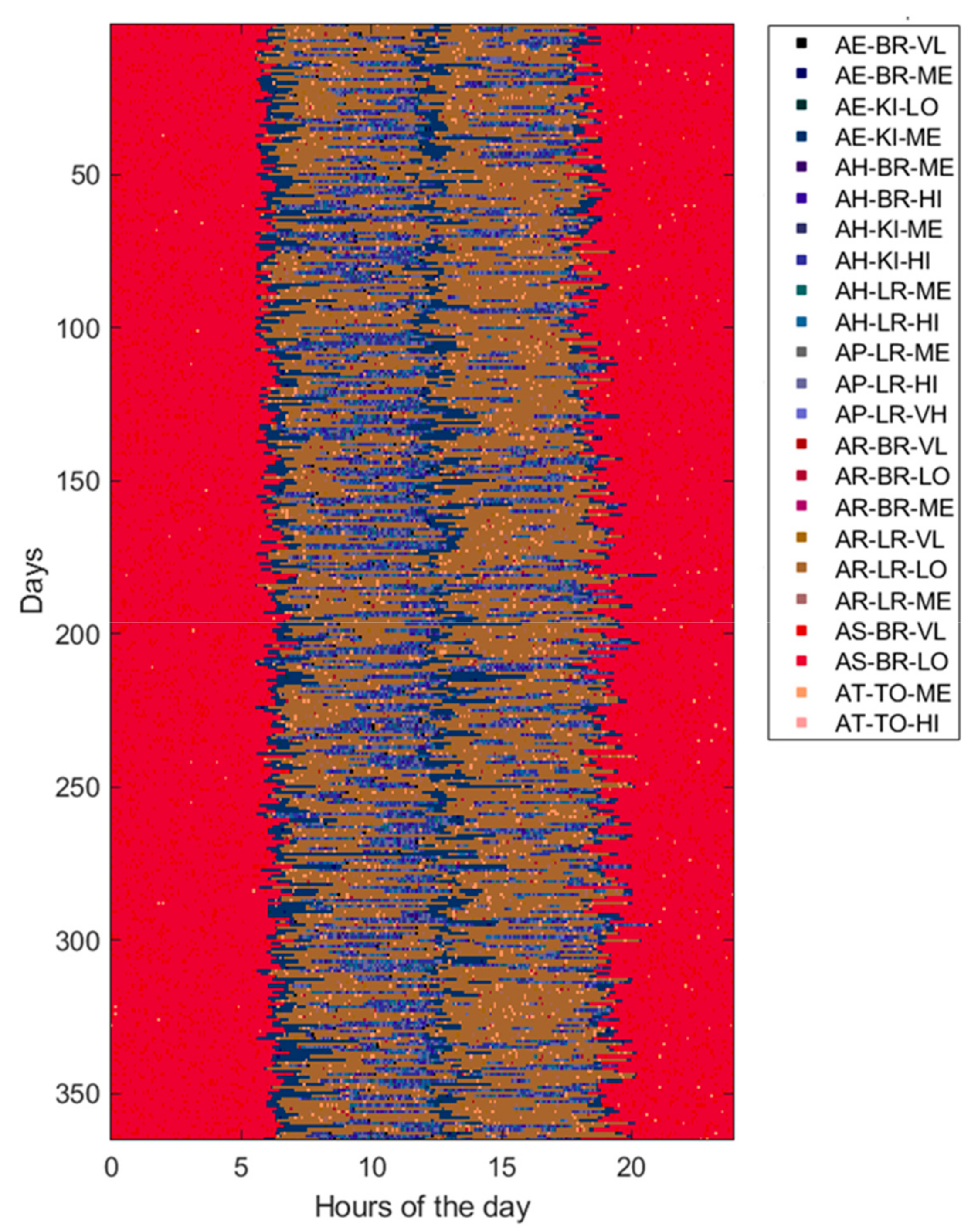
| Activity of Daily Living (ADL) | Home Location (LOC) | Heartrate Level (HRL) |
|---|---|---|
| Eating (AE) Housekeeping (AH) Physical exercise (AP) Resting (AR) Sleeping (AS) Toileting (AT) | Bedroom (BR) Kitchen (KI) Living room (LR) Toilet (TO) | Very low (VL) [<50 beats/min] Low (LO) [65–80 beats/min] Medium (ME) [80–95 beats/min] High (HI) [95–110 beats/min] Very high (VH) [>110 beats/min] |
© 2019 by the authors. Licensee MDPI, Basel, Switzerland. This article is an open access article distributed under the terms and conditions of the Creative Commons Attribution (CC BY) license (http://creativecommons.org/licenses/by/4.0/).
Share and Cite
Diraco, G.; Leone, A.; Siciliano, P. AI-Based Early Change Detection in Smart Living Environments. Sensors 2019, 19, 3549. https://doi.org/10.3390/s19163549
Diraco G, Leone A, Siciliano P. AI-Based Early Change Detection in Smart Living Environments. Sensors. 2019; 19(16):3549. https://doi.org/10.3390/s19163549
Chicago/Turabian StyleDiraco, Giovanni, Alessandro Leone, and Pietro Siciliano. 2019. "AI-Based Early Change Detection in Smart Living Environments" Sensors 19, no. 16: 3549. https://doi.org/10.3390/s19163549
APA StyleDiraco, G., Leone, A., & Siciliano, P. (2019). AI-Based Early Change Detection in Smart Living Environments. Sensors, 19(16), 3549. https://doi.org/10.3390/s19163549