Figure 1.
Prototyping of smart objects (a cup, a toothbrush, and a fork), whose orientation and movement data are collected and sent in real time by an inertial miniature board (The Tactigon).
Figure 1.
Prototyping of smart objects (a cup, a toothbrush, and a fork), whose orientation and movement data are collected and sent in real time by an inertial miniature board (The Tactigon).
Figure 2.
Architecture for connecting heterogeneous devices. Binary, location, and inertial board sensors send raw data to gateways, which collect, aggregate, and publish data with MQTT in JSON format. The Android Wear application collects, aggregates, and publishes the data directly using MQTT through WiFi connection.
Figure 3.
Fuzzy fusion of spatial-temporal features of sensors: (i) data from the heterogeneous sensors are distributed in real time; (ii) fuzzy logic processes spatial-temporal features; (iii) a light and efficient classifier learns activities from the features.
Figure 3.
Fuzzy fusion of spatial-temporal features of sensors: (i) data from the heterogeneous sensors are distributed in real time; (ii) fuzzy logic processes spatial-temporal features; (iii) a light and efficient classifier learns activities from the features.
Figure 4.
Example of the fuzzy scale defined for on distance to the location sensor. Example degrees for values evaluating the distances .
Figure 4.
Example of the fuzzy scale defined for on distance to the location sensor. Example degrees for values evaluating the distances .
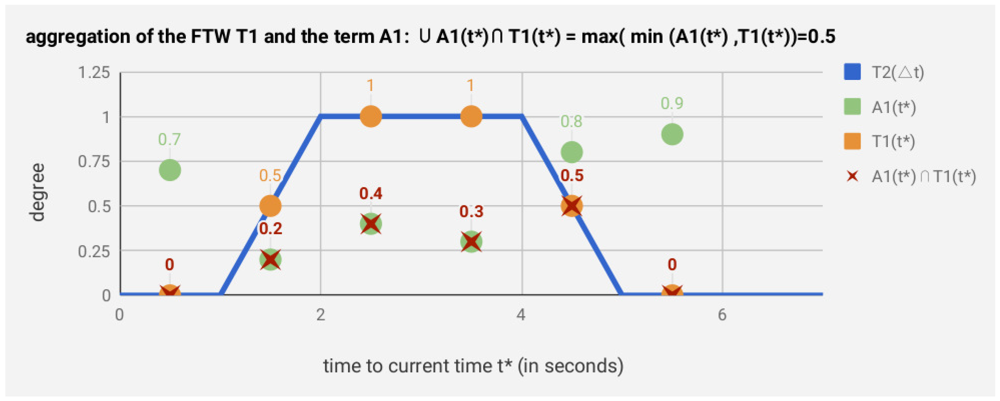
Figure 5.
Example of temporal aggregation of the FTW [1 s, 2 s, 4 s, 5 s] (in magnitude of seconds s) for the degrees of the term . The aggregation degree is determined by the max-min operator. The value defines a fuzzy spatial temporal feature of the sensor stream.
Figure 5.
Example of temporal aggregation of the FTW [1 s, 2 s, 4 s, 5 s] (in magnitude of seconds s) for the degrees of the term . The aggregation degree is determined by the max-min operator. The value defines a fuzzy spatial temporal feature of the sensor stream.
Figure 6.
Data from heterogeneous sensors. The top-left shows the location in meters from a UWB device. The top-right shows acceleration from a wearable device. The bottom-left shows acceleration in the inhabitant’s cup. The bottom-right shows the activation of the microwave. Some inhabitant behaviors and the impact on sensors are indicated in the timelines.
Figure 7.
Confusion matrix for the best classifiers. (A) SVM + in the baseline, (B) KNN + with fuzzy spatial features, and (C) KNN + with fuzzy spatial temporal features.
Figure 7.
Confusion matrix for the best classifiers. (A) SVM + in the baseline, (B) KNN + with fuzzy spatial features, and (C) KNN + with fuzzy spatial temporal features.
Table 1.
Sequence activities of the case scenes.
Table 1.
Sequence activities of the case scenes.
| Scene 1 | Sleep → Toilet → Prepare lunch → Eat → Watch TV → Phone → Dressing → Toothbrush → Exit |
| Scene 2 | Enter → Drinking → Toilet → Phone → Exit |
| Scene 3 | Enter → Drinking → Toilet → Dressing → Cooking → Eat → Sleep |
| Scene 4 | Enter → Toilet → Dressing → Watching TV → Cooking → Eat → Toothbrush → Sleep |
| Scene 5 | Enter → Drinking → Toilet → Dressing → Cooking → Eat → Phone → Toothbrush → Sleep |
Table 2.
Frequency (number of time-steps) for each activity and scene.
Table 2.
Frequency (number of time-steps) for each activity and scene.
| Activity | Scene 1 | Scene 2 | Scene 3 | Scene 4 | Scene 5 |
|---|
| Sleep | 10 | 0 | 16 | 11 | 11 |
| Toilet | 13 | 10 | 6 | 10 | 14 |
| Cooking | 29 | 0 | 27 | 17 | 24 |
| Eat | 36 | 0 | 40 | 46 | 41 |
| Watch TV | 20 | 0 | 0 | 16 | 0 |
| Phone | 14 | 17 | 0 | 0 | 15 |
| Dressing | 15 | 0 | 21 | 16 | 17 |
| Toothbrush | 21 | 0 | 0 | 18 | 18 |
| Exit | 3 | 2 | 0 | 0 | 0 |
| Enter | 0 | 3 | 4 | 2 | 3 |
| Drinking | 0 | 16 | 7 | 0 | 12 |
Table 3.
Results with baseline features: precision (Pre), recall (Rec) and F1-score (F1-sc).
Table 3.
Results with baseline features: precision (Pre), recall (Rec) and F1-score (F1-sc).
| SVM | kNN | C4.5 |
| Activity | Pre | Acc | F1-sc | Pre | Acc | F1-sc | Pre | Acc | F1-sc |
| Sleep | 94.73 | 77.08 | 85.00 | 94.73 | 77.08 | 85.00 | 65.45 | 83.33 | 73.31 |
| Toilet | 95.83 | 54.71 | 69.66 | 68.75 | 88.67 | 77.45 | 86.27 | 90.56 | 88.36 |
| Cooking | 66.38 | 89.69 | 76.29 | 58.02 | 75.25 | 65.52 | 50.48 | 67.01 | 57.08 |
| Eating | 81.43 | 92.02 | 86.40 | 80.36 | 93.86 | 86.59 | 76.97 | 77.30 | 77.13 |
| Watching TV | 100 | 94.44 | 97.14 | 94.73 | 94.44 | 94.59 | 91.17 | 91.66 | 91.42 |
| Phone | 100 | 93.47 | 96.62 | 100 | 100 | 100 | 97.22 | 95.65 | 96.43 |
| Dressing | 90.00 | 94.20 | 92.05 | 93.24 | 97.10 | 95.13 | 88.00 | 76.81 | 82.02 |
| Brushing Teeth | 97.36 | 73.68 | 83.88 | 76.27 | 89.47 | 82.34 | 70.96 | 50.87 | 59.26 |
| Drinking | 56.25 | 45.71 | 50.43 | 32.25 | 57.14 | 41.23 | 32.85 | 80.00 | 46.58 |
| Enter/Exit | 100 | 88.23 | 93.75 | 78.94 | 94.11 | 85.86 | 86.66 | 94.11 | 90.23 |
| Average | 88.20 | 80.32 | 83.12 | 77.73 | 86.71 | 81.37 | 74.60 | 80.73 | 76.23 |
| SVM | kNN | C4.5 |
| Activity | Pre | Acc | F1-sc | Pre | Acc | F1-sc | Pre | Acc | F1-sc |
| Sleep | 90.47 | 77.08 | 83.24 | 90.47 | 77.08 | 83.24 | 75.00 | 56.25 | 64.28 |
| Toilet | 66.67 | 64.15 | 65.38 | 72.13 | 88.67 | 79.55 | 64.06 | 83.01 | 72.31 |
| Cooking | 80.95 | 87.62 | 84.15 | 63.88 | 61.85 | 62.85 | 63.63 | 56.70 | 59.96 |
| Eating | 84.65 | 93.86 | 89.02 | 82.53 | 92.02 | 87.01 | 88.28 | 71.16 | 78.80 |
| Watching TV | 94.87 | 97.22 | 96.03 | 94.87 | 97.22 | 96.03 | 47.05 | 36.11 | 40.86 |
| Phone | 94.44 | 100 | 97.14 | 97.72 | 93.47 | 95.55 | 97.82 | 93.47 | 95.60 |
| Dressing | 94.73 | 100 | 97.29 | 90.36 | 100 | 94.93 | 84.61 | 68.11 | 75.47 |
| Brushing Teeth | 82.22 | 68.42 | 74.68 | 73.91 | 71.92 | 72.90 | 93.87 | 84.21 | 88.78 |
| Drinking | 34.61 | 28.57 | 31.30 | 22.85 | 28.57 | 25.39 | 38.15 | 85.71 | 52.80 |
| Enter/Exit | 89.47 | 82.35 | 85.76 | 89.47 | 100 | 94.44 | 76.00 | 100 | 86.36 |
| Average | 81.31 | 79.92 | 80.40 | 77.82 | 81.08 | 79.19 | 72.85 | 73.47 | 71.52 |
| SVM | kNN | C4.5 |
| Activity | Pre | Acc | F1-sc | Pre | Acc | F1-sc | Pre | Acc | F1-sc |
| Sleep | 90.47 | 77.08 | 83.24 | 90.90 | 77.08 | 83.42 | 92.85 | 29.16 | 44.39 |
| Toilet | 66.10 | 71.69 | 68.78 | 67.18 | 86.79 | 75.74 | 82.05 | 64.15 | 72.00 |
| Cooking | 78.21 | 85.56 | 81.72 | 73.03 | 79.38 | 76.07 | 45.78 | 52.57 | 48.94 |
| Eating | 89.01 | 94.47 | 91.66 | 87.57 | 93.25 | 90.32 | 91.83 | 58.89 | 71.76 |
| Watching TV | 88.09 | 100 | 93.67 | 77.78 | 77.78 | 77.78 | 79.16 | 100 | 88.37 |
| Phone | 95.74 | 93.47 | 94.59 | 97.56 | 86.95 | 91.95 | 85.41 | 86.95 | 86.17 |
| Dressing | 92.95 | 94.20 | 93.57 | 93.05 | 95.65 | 94.33 | 75.00 | 62.31 | 68.07 |
| Brushing Teeth | 86.20 | 87.71 | 86.95 | 80.00 | 77.19 | 78.57 | 64.38 | 84.21 | 79.97 |
| Drinking | 58.33 | 40.00 | 47.45 | 48.14 | 40.00 | 43.69 | 30.00 | 74.28 | 42.73 |
| Enter/Exit | 0 | 0 | 0 | 71.42 | 64.70 | 67.90 | 69.23 | 47.05 | 56.03 |
| Average | 74.51 | 74.42 | 74.46 | 78.67 | 77.87 | 78.27 | 71.57 | 65.96 | 68.65 |
| Learning Time | SVM | kNN | C4.5 |
| Average time in mobile device (in ms) | 998 | 25 | 1980 |
Table 4.
Results with fuzzy features (spatial): precision (Pre), recall (Rec) and F1-score (F1-sc).
Table 4.
Results with fuzzy features (spatial): precision (Pre), recall (Rec) and F1-score (F1-sc).
| SVM | kNN | C4.5 |
| Activity | Pre | Acc | F1-sc | Pre | Acc | F1-sc | Pre | Acc | F1-sc |
| Sleep | 90.24 | 77.08 | 83.14 | 92.30 | 77.08 | 84.01 | 79.62 | 91.66 | 85.22 |
| Toilet | 84.90 | 86.79 | 85.83 | 89.58 | 84.90 | 87.18 | 88.00 | 92.45 | 90.17 |
| Cooking | 63.02 | 86.59 | 72.95 | 60.97 | 73.19 | 66.52 | 44.71 | 75.25 | 56.09 |
| Eating | 90.38 | 91.41 | 90.89 | 82.05 | 92.63 | 87.02 | 85.08 | 71.77 | 77.86 |
| Watching TV | 100 | 94.44 | 97.14 | 97.05 | 94.44 | 95.73 | 96.96 | 91.66 | 94.24 |
| Phone | 100 | 91.30 | 95.45 | 100 | 95.65 | 97.77 | 87.17 | 93.47 | 90.21 |
| Dressing | 93.15 | 98.55 | 95.77 | 83.75 | 97.10 | 89.93 | 73.21 | 73.91 | 73.56 |
| Brushing Teeth | 95.74 | 82.45 | 88.60 | 86.27 | 91.22 | 88.68 | 83.67 | 82.45 | 83.06 |
| Drinking | 50.00 | 71.42 | 58.82 | 44.73 | 62.85 | 52.27 | 32.14 | 77.14 | 45.37 |
| Enter/Exit | 100 | 88.23 | 93.75 | 82.35 | 94.11 | 87.84 | 55.55 | 94.11 | 69.86 |
| Average | 86.74 | 86.83 | 86.23 | 81.90 | 86.32 | 83.69 | 72.61 | 84.39 | 76.56 |
| SVM | kNN | C4.5 |
| Activity | Pre | Acc | F1-sc | Pre | Acc | F1-sc | Pre | Acc | F1-sc |
| Sleep | 92.68 | 77.08 | 84.16 | 86.66 | 77.08 | 81.59 | 75.00 | 68.75 | 71.73 |
| Toilet | 71.66 | 83.01 | 76.92 | 91.11 | 79.24 | 84.76 | 88.09 | 71.69 | 79.05 |
| Cooking | 79.79 | 91.75 | 85.35 | 79.74 | 83.50 | 81.58 | 54.71 | 40.20 | 46.35 |
| Eating | 94.80 | 92.63 | 93.70 | 87.80 | 93.86 | 90.73 | 87.96 | 62.57 | 73.12 |
| Watching TV | 94.87 | 97.22 | 96.03 | 94.87 | 97.22 | 96.03 | 97.22 | 94.44 | 95.81 |
| Phone | 95.65 | 93.47 | 94.55 | 95.45 | 91.30 | 93.33 | 97.95 | 100 | 98.96 |
| Dressing | 89.61 | 100 | 94.52 | 87.65 | 98.55 | 92.78 | 68.25 | 69.56 | 68.90 |
| Brushing Teeth | 88.46 | 84.21 | 86.28 | 85.45 | 85.96 | 85.70 | 78.00 | 68.42 | 72.89 |
| Drinking | 57.14 | 62.85 | 59.86 | 58.06 | 60.00 | 59.01 | 24.07 | 80.00 | 37.01 |
| Enter/Exit | 90.00 | 100 | 94.73 | 87.50 | 82.35 | 84.84 | 77.27 | 100 | 87.17 |
| Average | 85.46 | 88.22 | 86.61 | 85.43 | 84.90 | 85.03 | 74.85 | 75.56 | 73.10 |
| SVM | kNN | C4.5 |
| Activity | Pre | Acc | F1-sc | Pre | Acc | F1-sc | Pre | Acc | F1-sc |
| Sleep | 87.17 | 72.91 | 79.41 | 92.30 | 95.83 | 94.03 | 81.39 | 72.91 | 76.92 |
| Toilet | 63.79 | 69.81 | 66.66 | 77.04 | 90.56 | 83.26 | 66.66 | 75.47 | 70.79 |
| Cooking | 81.72 | 88.65 | 85.04 | 80.88 | 73.19 | 76.84 | 61.67 | 45.36 | 52.27 |
| Eating | 94.00 | 90.18 | 92.05 | 90.96 | 93.25 | 92.09 | 88.88 | 55.21 | 68.11 |
| Watching TV | 92.68 | 100 | 96.20 | 88.88 | 100 | 94.11 | 92.85 | 100 | 96.29 |
| Phone | 97.91 | 97.82 | 97.87 | 97.95 | 100 | 98.96 | 100 | 67.39 | 80.51 |
| Dressing | 92.75 | 95.65 | 94.18 | 90.27 | 95.65 | 92.88 | 88.09 | 55.07 | 67.77 |
| Brushing Teeth | 86.95 | 73.68 | 79.77 | 84.74 | 91.22 | 87.86 | 72.72 | 19.29 | 30.50 |
| Drinking | 64.28 | 80.00 | 71.28 | 59.09 | 74.28 | 65.82 | 28.43 | 82.85 | 42.33 |
| Enter/Exit | 81.25 | 94.11 | 87.21 | 88.88 | 94.11 | 91.42 | 80.95 | 88.23 | 84.43 |
| Average | 84.25 | 86.28 | 85.25 | 85.10 | 90.81 | 87.86 | 76.16 | 66.18 | 70.82 |
| Learning Time | SVM | kNN | C4.5 |
| Average time in mobile device (in ms) | 2676 | 23 | 5382 |
Table 5.
Results with fuzzy features (spatial and temporal): precision (Pre), recall (Rec) and F1-score (F1-sc).
Table 5.
Results with fuzzy features (spatial and temporal): precision (Pre), recall (Rec) and F1-score (F1-sc).
| SVM | kNN | C4.5 |
| Activity | Pre | Acc | F1-sc | Pre | Acc | F1-sc | Pre | Acc | F1-sc |
| Sleep | 90.24 | 77.08 | 83.14 | 92.30 | 77.08 | 84.01 | 79.62 | 91.66 | 85.22 |
| Toilet | 84.90 | 86.79 | 85.83 | 89.58 | 84.90 | 87.18 | 88.00 | 92.45 | 90.17 |
| Cooking | 63.02 | 86.59 | 72.95 | 60.97 | 73.19 | 66.52 | 44.71 | 75.25 | 56.09 |
| Eating | 90.38 | 91.41 | 90.89 | 82.05 | 92.63 | 87.02 | 85.08 | 71.77 | 77.86 |
| Watching TV | 100 | 94.44 | 97.14 | 97.05 | 94.44 | 95.73 | 96.96 | 91.66 | 94.24 |
| Phone | 100 | 91.30 | 95.45 | 100 | 95.65 | 97.77 | 87.17 | 93.47 | 90.21 |
| Dressing | 93.15 | 98.55 | 95.77 | 83.75 | 97.10 | 89.93 | 73.21 | 73.91 | 73.56 |
| Brushing Teeth | 95.74 | 82.45 | 88.60 | 86.27 | 91.22 | 88.68 | 83.67 | 82.45 | 83.06 |
| Drinking | 50.00 | 71.42 | 58.82 | 44.73 | 62.85 | 52.27 | 32.14 | 77.14 | 45.37 |
| Enter/Exit | 100 | 88.23 | 93.75 | 82.35 | 94.11 | 87.84 | 55.55 | 94.11 | 69.86 |
| Average | 86.74 | 86.83 | 86.23 | 81.90 | 86.32 | 83.69 | 72.61 | 84.39 | 76.56 |
| SVM | kNN | C4.5 |
| Activity | Pre | Acc | F1-sc | Pre | Acc | F1-sc | Pre | Acc | F1-sc |
| Sleep | 93.02 | 89.58 | 91.27 | 91.83 | 93.75 | 92.78 | 59.25 | 66.66 | 62.74 |
| Toilet | 84.09 | 75.47 | 79.54 | 85.10 | 77.35 | 81.04 | 71.87 | 47.16 | 56.95 |
| Cooking | 94.38 | 91.75 | 93.04 | 94.56 | 93.81 | 94.18 | 72.09 | 40.20 | 51.62 |
| Eating | 97.87 | 86.50 | 91.83 | 90.11 | 93.25 | 91.65 | 83.69 | 58.89 | 69.13 |
| Watching TV | 90.00 | 75.00 | 81.81 | 95.23 | 100 | 97.56 | 91.66 | 55.55 | 69.18 |
| Phone | 97.82 | 95.65 | 96.72 | 92.45 | 100 | 96.07 | 100 | 100 | 100 |
| Dressing | 95.65 | 97.10 | 96.37 | 93.93 | 92.75 | 93.34 | 83.67 | 57.97 | 68.49 |
| Brushing Teeth | 87.23 | 73.68 | 79.88 | 89.28 | 89.47 | 89.37 | 35.96 | 68.42 | 47.14 |
| Drinking | 75.67 | 77.14 | 76.40 | 80.55 | 80.00 | 80.27 | 27.38 | 65.71 | 38.65 |
| Enter/Exit | 100 | 100 | 100 | 73.07 | 100 | 84.44 | 100 | 82.35 | 90.32 |
| Average | 91.57 | 86.18 | 88.80 | 88.61 | 92.04 | 90.29 | 72.56 | 64.29 | 68.17 |
| Learning Time | SVM | kNN | C4.5 |
| Average time in mobile device (in ms) | 2128 | 24 | 4308.5 |
Table 6.
Results with extended baseline features: precision (Pre), recall (Rec) and F1-score (F1-sc).
Table 6.
Results with extended baseline features: precision (Pre), recall (Rec) and F1-score (F1-sc).
| SVM | kNN | C4.5 |
| Activity | Pre | Acc | F1-sc | Pre | Acc | F1-sc | Pre | Acc | F1-sc |
| Sleep | 84.44 | 77.08 | 80.59 | 77.08 | 77.08 | 77.08 | 80.64 | 56.25 | 66.27 |
| Toilet | 78.57 | 62.26 | 69.47 | 67.85 | 79.24 | 73.11 | 93.02 | 86.79 | 89.79 |
| Cooking | 76.04 | 84.53 | 80.06 | 68.57 | 69.07 | 68.82 | 55.20 | 82.47 | 66.13 |
| Eating | 85.22 | 95.09 | 89.88 | 81.81 | 93.25 | 87.16 | 85.71 | 77.30 | 81.29 |
| Watching TV | 94.73 | 94.44 | 94.59 | 85.71 | 94.44 | 89.86 | 97.14 | 94.44 | 95.77 |
| Phone | 100 | 91.30 | 95.45 | 100 | 93.47 | 96.62 | 78.18 | 93.47 | 85.14 |
| Dressing | 92.10 | 100 | 95.89 | 86.58 | 100 | 92.81 | 86.41 | 100 | 92.71 |
| Brushing Teeth | 88.63 | 74.54 | 80.98 | 69.64 | 78.18 | 73.66 | 66.67 | 47.27 | 55.31 |
| Drinking | 74.19 | 76.47 | 75.31 | 61.22 | 94.11 | 74.18 | 43.28 | 91.17 | 58.70 |
| Enter/Exit | 84.61 | 88.23 | 86.38 | 84.21 | 94.11 | 88.88 | 80.00 | 94.11 | 86.48 |
| Average | 85.85 | 84.39 | 84.86 | 78.27 | 87.29 | 82.22 | 76.62 | 82.33 | 77.76 |
| SVM | kNN | C4.5 |
| Activity | Pre | Acc | F1-sc | Pre | Acc | F1-sc | Pre | Acc | F1-sc |
| Sleep | 86.66 | 87.50 | 87.08 | 82.69 | 91.66 | 86.94 | 76.74 | 68.75 | 72.52 |
| Toilet | 83.78 | 58.49 | 68.88 | 93.61 | 83.01 | 88.00 | 80.48 | 62.26 | 70.21 |
| Cooking | 88.37 | 86.59 | 87.47 | 91.02 | 82.47 | 86.53 | 57.30 | 65.97 | 61.33 |
| Eating | 95.27 | 90.79 | 92.98 | 88.63 | 95.09 | 91.75 | 85.57 | 61.96 | 71.88 |
| Watching TV | 85.00 | 94.44 | 89.47 | 85.71 | 97.22 | 91.10 | 82.85 | 86.11 | 84.45 |
| Phone | 97.72 | 93.47 | 95.55 | 93.75 | 95.65 | 94.69 | 100 | 100 | 100 |
| Dressing | 94.20 | 98.55 | 96.32 | 85.18 | 98.55 | 91.38 | 94.24 | 94.20 | 93.30 |
| Brushing Teeth | 91.48 | 90.90 | 91.19 | 86.67 | 87.27 | 87.97 | 87.17 | 69.09 | 77.08 |
| Drinking | 85.71 | 94.11 | 89.71 | 86.48 | 97.05 | 91.46 | 55.31 | 91.17 | 68.85 |
| Enter/Exit | 95.00 | 100 | 97.43 | 79.16 | 100 | 88.37 | 100 | 100 | 100 |
| Average | 90.32 | 89.48 | 89.90 | 87.49 | 92.80 | 90.07 | 81.78 | 79.95 | 80.86 |
| SVM | kNN | C4.5 |
| Activity | Pre | Acc | F1-sc | Pre | Acc | F1-sc | Pre | Acc | F1-sc |
| Sleep | 84.61 | 68.75 | 75.86 | 88.67 | 95.83 | 92.11 | 64.00 | 66.66 | 65.30 |
| Toilet | 92.50 | 71.69 | 80.78 | 90.69 | 75.47 | 82.38 | 84.44 | 77.35 | 80.74 |
| Cooking | 95.45 | 89.69 | 92.48 | 95.23 | 86.59 | 90.71 | 49.07 | 56.70 | 52.71 |
| Eating | 96.07 | 90.18 | 93.03 | 89.28 | 92.02 | 90.63 | 71.83 | 37.42 | 49.20 |
| Watching TV | 94.44 | 94.44 | 94.44 | 86.04 | 100 | 92.49 | 100 | 44.44 | 61.53 |
| Phone | 100 | 93.47 | 96.62 | 90.38 | 100 | 94.94 | 100 | 100 | 100 |
| Dressing | 94.52 | 97.10 | 95.79 | 89.85 | 92.75 | 91.28 | 95.23 | 62.31 | 75.33 |
| Brushing Teeth | 89.74 | 63.63 | 74.46 | 92.45 | 90.90 | 91.67 | 73.80 | 56.36 | 63.91 |
| Drinking | 97.05 | 100 | 98.50 | 81.17 | 100 | 93.15 | 76.19 | 94.11 | 84.21 |
| Enter/Exit | 100 | 100 | 100 | 82.60 | 100 | 90.47 | 100 | 82.35 | 90.32 |
| Average | 94.44 | 86.89 | 90.51 | 89.24 | 93.35 | 91.25 | 81.45 | 67.74 | 73.98 |
Table 7.
S1: Non Binary (inertial + location) sensors. S2: non-location (binary + inertial), S3: non-inertial (binary + location), S4: only inertial.
Table 7.
S1: Non Binary (inertial + location) sensors. S2: non-location (binary + inertial), S3: non-inertial (binary + location), S4: only inertial.
| S1 | S2 |
| Activity | Pre | Acc | F1-sc | Pre | Acc | F1-sc |
| Sleep | 91.30 | 89.58 | 90.43 | 85.71 | 91.66 | 88.59 |
| Toilet | 76.47 | 66.03 | 70.98 | 90.90 | 77.35 | 83.58 |
| Cooking | 92.68 | 82.47 | 87.28 | 93.75 | 80.41 | 86.57 |
| Eating | 91.19 | 90.79 | 90.99 | 90.06 | 92.63 | 91.33 |
| Watching TV | 92.30 | 97.22 | 94.70 | 83.33 | 97.22 | 89.74 |
| Phone | 90.19 | 97.82 | 93.85 | 87.03 | 100 | 93.06 |
| Dressing | 71.01 | 79.71 | 75.11 | 88.00 | 97.10 | 92.32 |
| Brushing Teeth | 92.59 | 90.90 | 91.74 | 91.11 | 81.81 | 86.21 |
| Drinking | 72.34 | 100 | 83.95 | 84.61 | 100 | 91.66 |
| Enter/Exit | 73.07 | 100 | 84.44 | 82.60 | 100 | 90.47 |
| Average | 84.34 | 89.45 | 86.82 | 87.71 | 91.82 | 89.72 |
| S3 | S4 |
| Activity | Pre | Acc | F1-sc | Pre | Acc | F1-sc |
| Sleep | 79.62 | 85.41 | 82.42 | 66.12 | 89.58 | 76.08 |
| Toilet | 76.92 | 75.47 | 76.19 | 47.54 | 60.37 | 53.19 |
| Cooking | 97.77 | 94.84 | 96.28 | 66.66 | 61.85 | 64.17 |
| Eating | 87.57 | 93.86 | 90.60 | 91.91 | 82.20 | 86.78 |
| Watching TV | 82.22 | 97.22 | 89.09 | 50.00 | 52.77 | 51.35 |
| Phone | 96.00 | 95.65 | 95.82 | 87.50 | 91.30 | 89.36 |
| Dressing | 88.31 | 97.10 | 92.49 | 38.59 | 39.13 | 38.86 |
| Brushing Teeth | 70.00 | 85.45 | 76.95 | 95.45 | 78.18 | 85.95 |
| Drinking | 100 | 97.05 | 98.50 | 49.18 | 97.05 | 65.28 |
| Enter/Exit | 90.47 | 100 | 94.99 | 81.25 | 82.35 | 81.79 |
| Average | 86.89 | 92.20 | 89.47 | 67.42 | 73.48 | 70.32 |


 ,
, 


