Deep Learning Convolutional Neural Network for the Retrieval of Land Surface Temperature from AMSR2 Data in China


 , ,
, ,
Abstract
1. Introduction
2. Study Area and Datasets
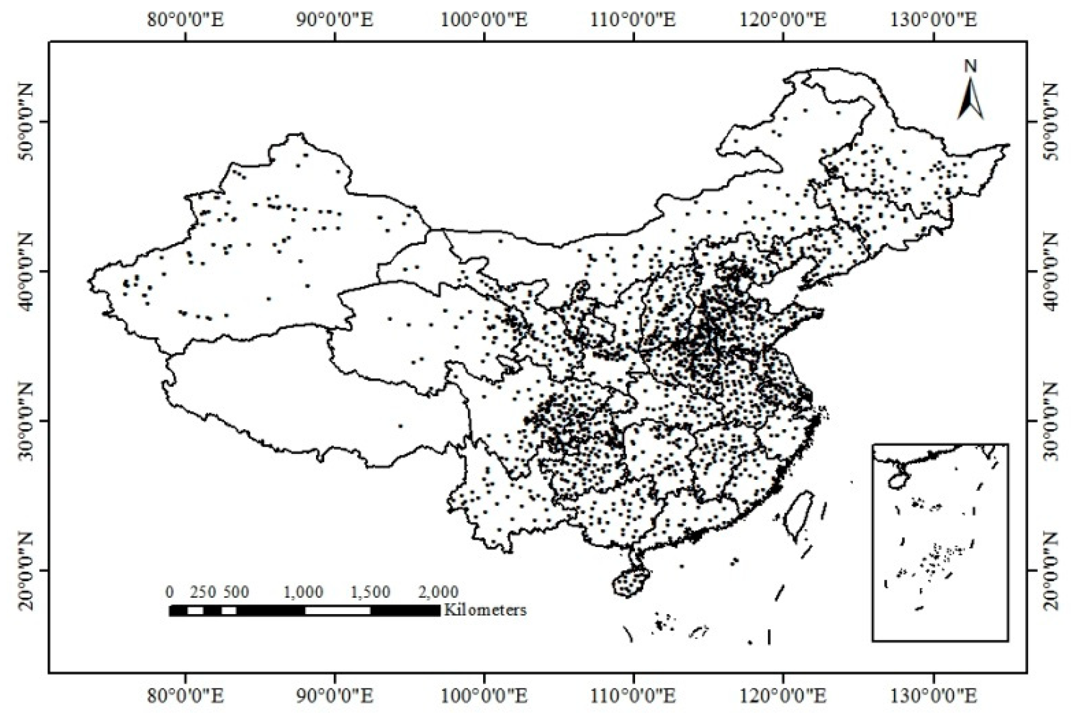
2.1. Study Area
2.2. Remote Sensing Data
2.3. Ground-Measured Data
3. Methods
3.1. Microwave Radiation Transmission Theory
3.2. CNN
4. Results
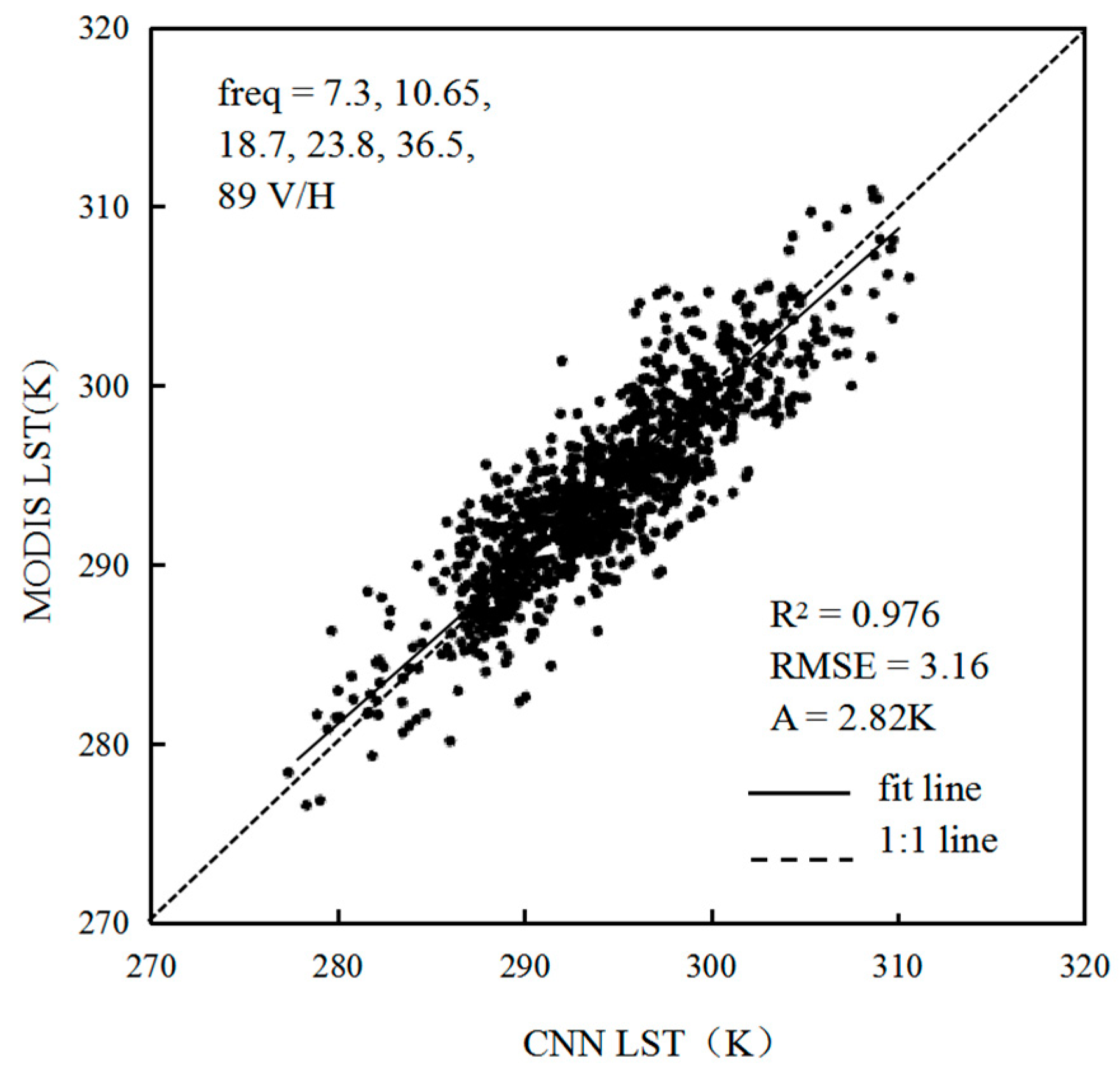
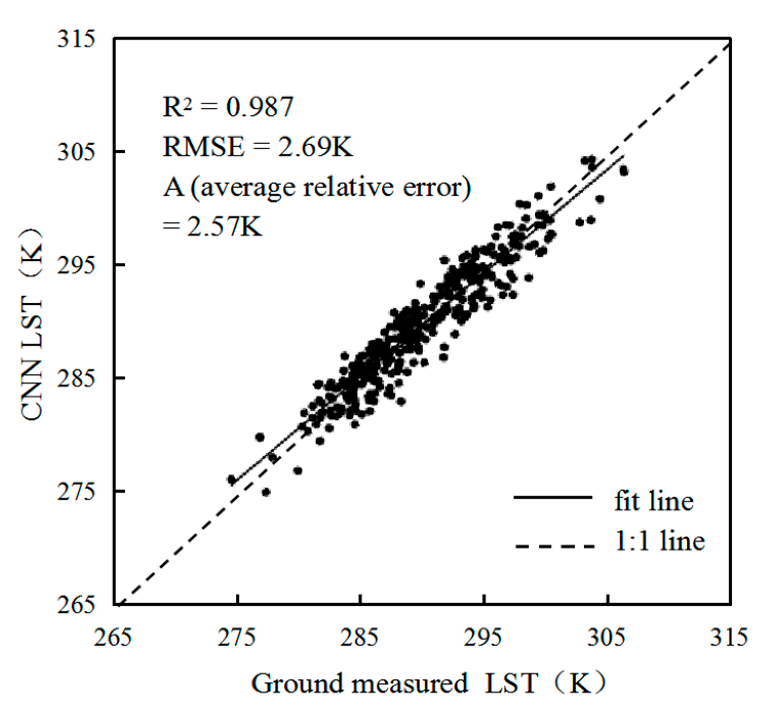
4.1. Analysis of CNN Retrieval Model Based on Different Channel Combinations
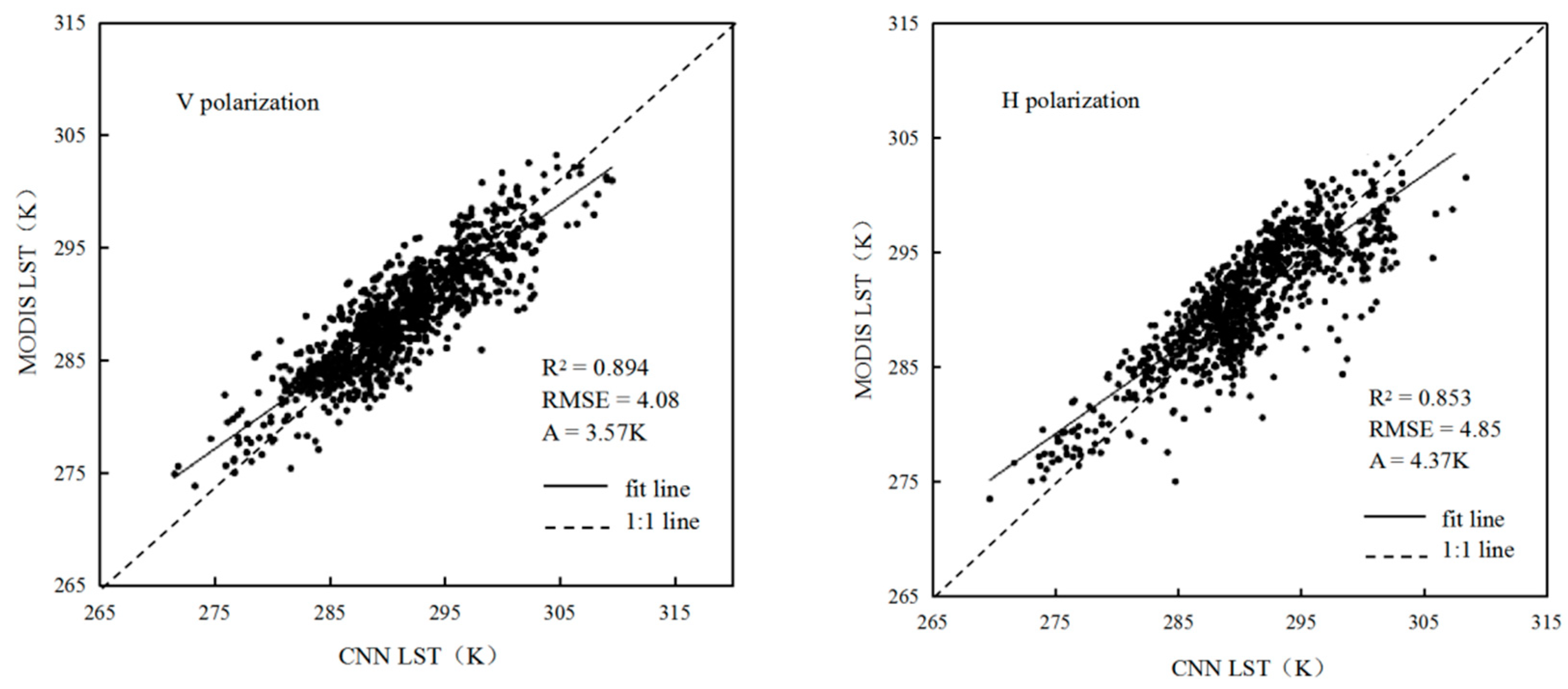
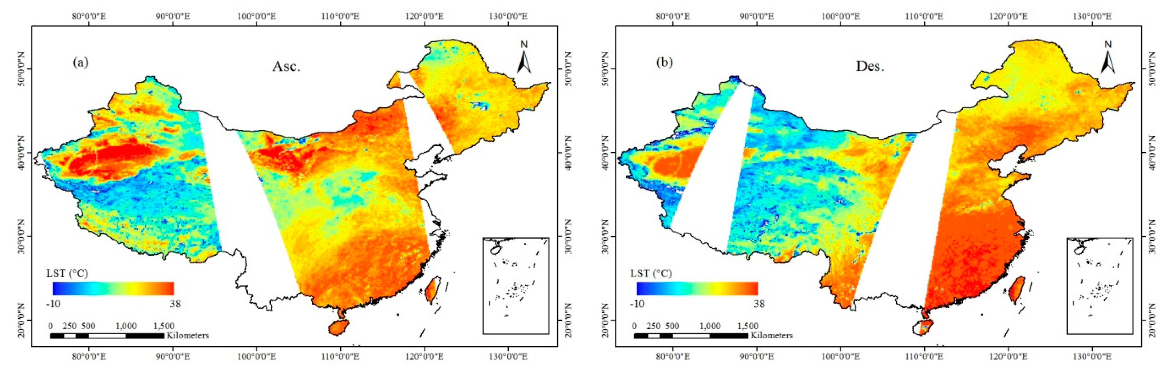
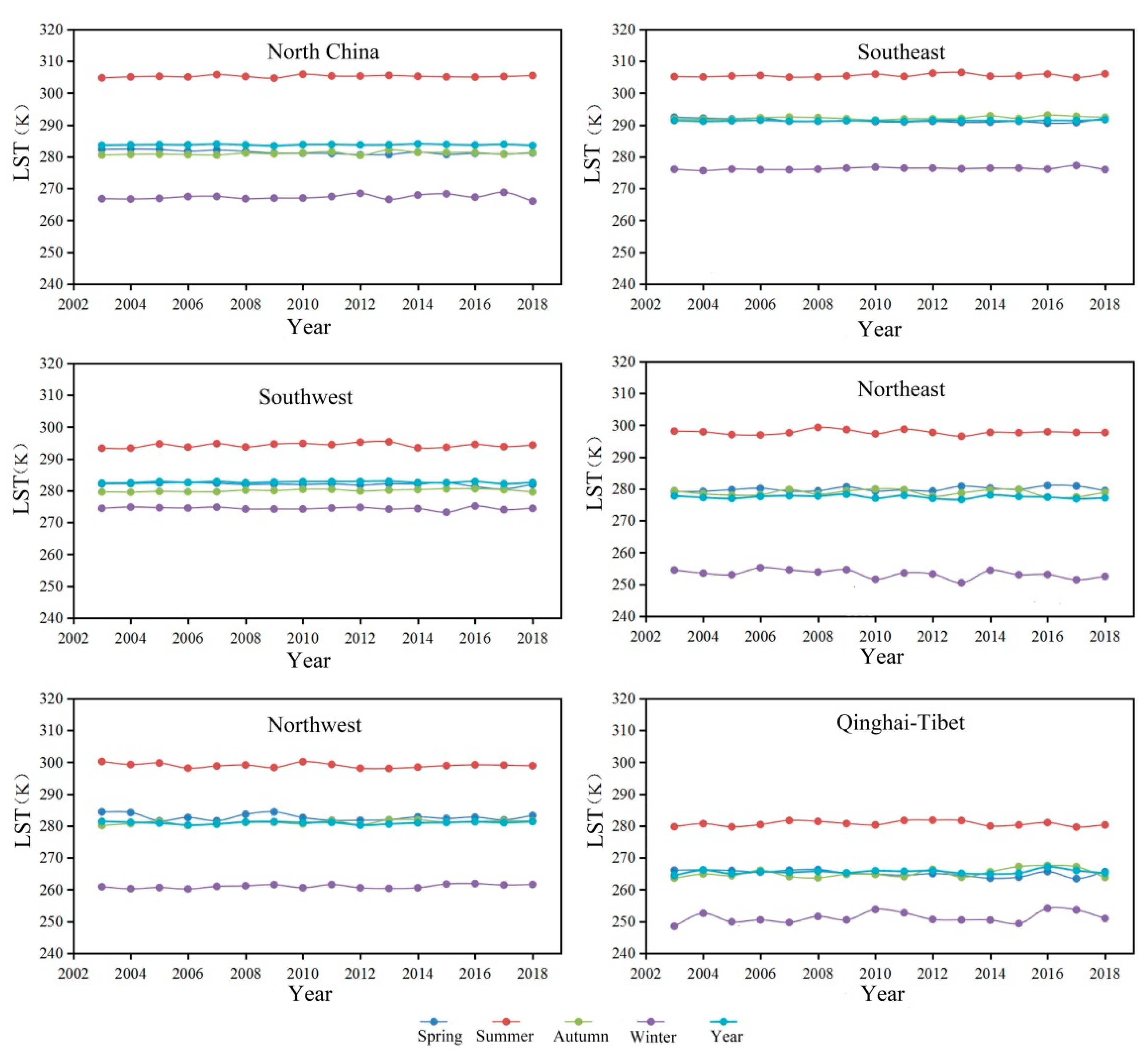
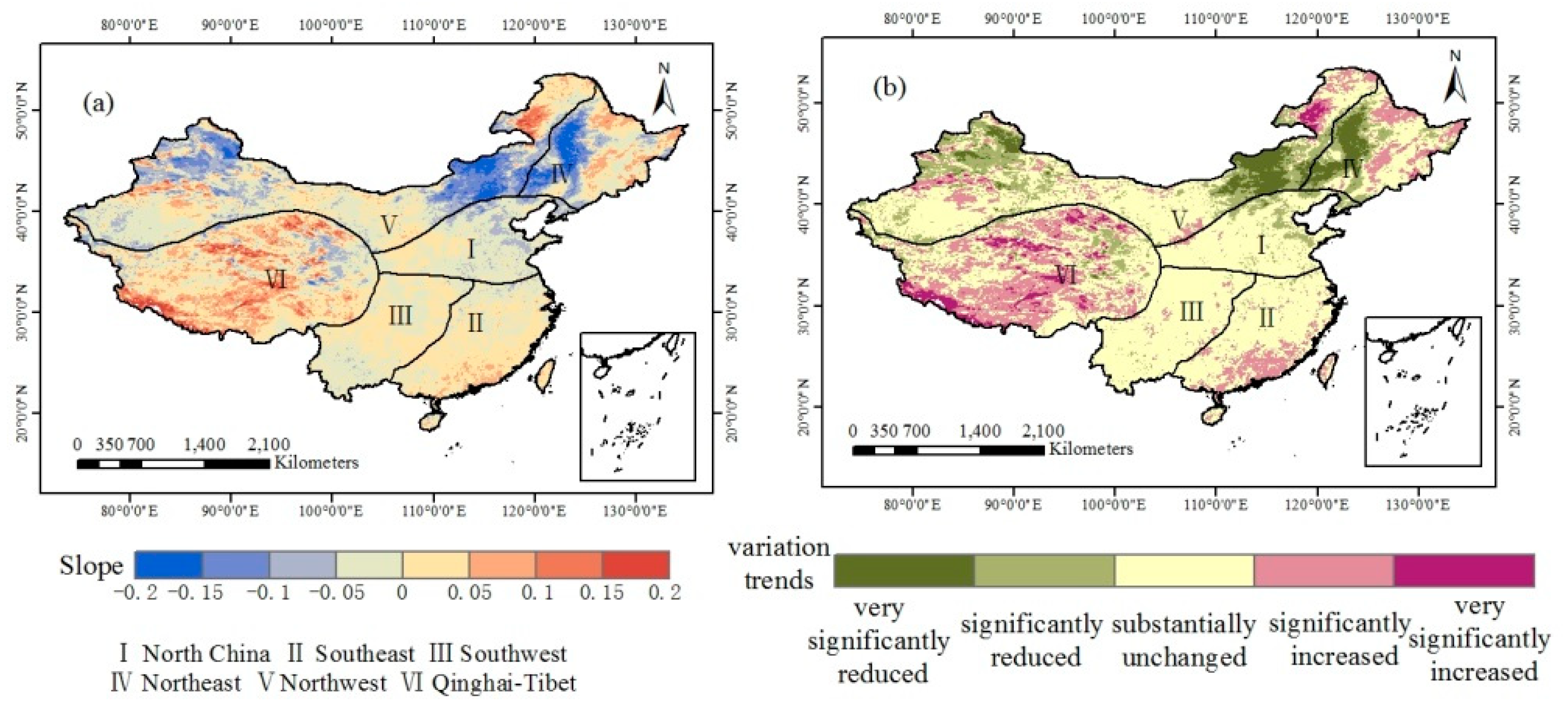
4.2. Analysis of CNN Retrieval Model based on Different Regions
4.3. Analysis of the CNN Retrieval model Based on Different Regions.
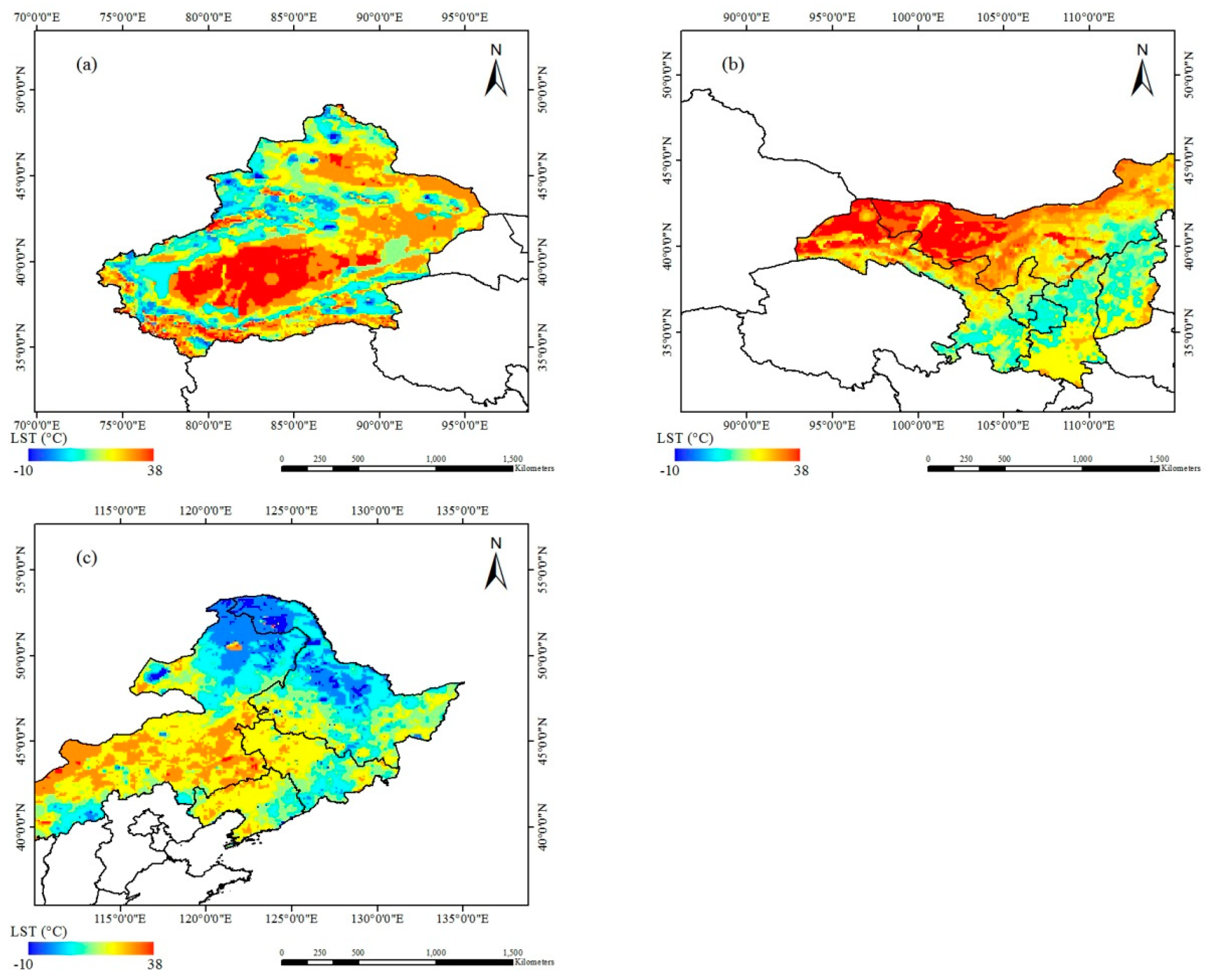
4.4. Spatiotemporal Variations in Summer Soil Moisture in China.
5. Discussion and Conclusions
Author Contributions
Funding
Conflicts of Interest
References
- Li, Z.L.; Tang, B.H.; Wu, H.; Ren, H.Z.; Yan, G.J.; Wan, Z.M.; Trigo, L.F.; Sobrino, J.C. Satellite-derived land surface temperature: Current status and perspectives. Remote Sens. Environ. 2013, 131, 14–37. [Google Scholar] [CrossRef]
- Kalma, J.D.; Mcvicar, T.R.; Mccabe, M.F. Estimating land surface evaporation: A review of methods using remotely sensed surface temperature data. Surv. Geophys. 2008, 29, 421–469. [Google Scholar] [CrossRef]
- Wang, K.C.; Li, Z.Q.; Cribb, M. Estimation of evaporative fraction from a combination of day and night land surface temperatures and NDVI: A new method to determine the Priestley–Taylor parameter. Remote Sens. Environ. 2006, 102, 293–305. [Google Scholar] [CrossRef]
- Coll, C.; Caselles, V.; Galve, J.M.; Valor, E.; Niclòs, R.; Sánchez-Tomás, J.M.; Rivas, R. Ground measurements for the validation of land surface temperatures derived from AATSR and MODIS data. Remote Sens. Environ. 2005, 97, 288–300. [Google Scholar] [CrossRef]
- Caselles, V.; Coll, C.; Valor, E. Land surface emissivity and temperature determination in the whole HAPEX-Sahel area from AVHRR data. Int. J. Remote Sens. 1997, 18, 1009–1027. [Google Scholar] [CrossRef]
- Jimenez-Munoz, J.C.; Cristobal, J.; Sobrino, J.A.; Barres, G.S.; Ninyerola, M.; Pons, X. Revision of the Single-Channel Algorithm for Land Surface Temperature Retrieval From Landsat Thermal-Infrared Data. IEEE Trans. Geosci. Remote Sens. 2008, 47, 339–349. [Google Scholar] [CrossRef]
- Liu, D.; Pu, R. Downscaling Thermal Infrared Radiance for Subpixel Land Surface Temperature Retrieval. Sensors 2008, 8, 2695–2706. [Google Scholar] [CrossRef]
- Wang, F.; Qin, Z.H.; Song, C.; Tu, L.; Karnieli, A.; Zhao, S. An improved mono-window algorithm for land surface temperature retrieval from landsat 8 thermal infrared sensor data. Remote Sens. 2015, 7, 4268–4289. [Google Scholar] [CrossRef]
- Duan, S.B.; Li, Z.L.; Wang, C.G.; Zhang, S.T.; Tang, B.H.; Leng, P.; Gao, M.F. Land-surface temperature retrieval from Landsat 8 single-channel thermal infrared data in combination with NCEP reanalysis data and ASTER GED product. Int. J. Remote Sens. 2018, 4, 1–16. [Google Scholar] [CrossRef]
- Prigent, C.; Aires, F.; Rossow, W.B. Land surface skin temperatures from a combined analysis of microwave and infrared satellite observations for an all-weather evaluation of the differences between air and skin temperatures. J. Geophys. Res. 2003, 108, 4310–4324. [Google Scholar] [CrossRef]
- Fily, M.; Royer, A.; Goïta, K.; Prigent, C. A simple retrieval method for land surface temperature and fraction of water surface determination from satellite microwave brightness temperatures in sub-arctic areas. Remote Sens. Environ. 2003, 85, 328–338. [Google Scholar] [CrossRef]
- Mao, K.B.; Shi, J.C.; Tang, H.J.; Li, Z.L.; Wang, X.F.; Chen, K.S. A Neural Network Technique for Separating Land Surface Emissivity and Temperature from ASTER Imagery. IEEE Trans. Geosci. Remote Sens. 2008, 46, 200–208. [Google Scholar] [CrossRef]
- Chen, X.Z.; Li, Y.; Han, L.S.; Su, Y.X.; Chen, S.S. Semi-empirical Model for Retrieving Land Surface Temperature Based on AMSR-E Data. Trop. Geogr. 2013, 33, 250–255. [Google Scholar]
- Maggioni, V.; Reichle, R.H.; Anagnostou, E.N. The effect of satellite rainfallerror modeling on soil moisture prediction uncertainty. J. Hydrometeorol. 2010, 12, 413–428. [Google Scholar] [CrossRef]
- Colliander, A.; Jackson, T.J.; Chan, S. Validation of SMAP surface soil moisture products with core validation sites. Remote Sens. Environ. 2017, 191, 215–231. [Google Scholar] [CrossRef]
- Kolassa, J.; Aires, F.; Polcher, J.; Prigent, C.; Jimenez, C.; Pereira, J.M.C. Soil moisture retrieval from multi-instrument observations: Information content analysis and retrieval methodology. J. Geophys. Res. Atmos. 2013, 118, 4847–4859. [Google Scholar] [CrossRef]
- Mcfarland, M.J.; Miller, R.L.; Neale, C.M.U. Land surface temperature derived from the ssm/i passive microwave brightness temperatures. IEEE Trans. Geosci. Remote Sens. 1990, 28, 839–845. [Google Scholar] [CrossRef]
- Njoku, E.G.; Li, L. Retrieval of land surface parameters using passive microwave measurements at 6–18 GHz. IEEE Trans. Geosci. Remote Sens. 1999, 37, 79–93. [Google Scholar] [CrossRef]
- Mao, K.B.; Shi, J.C.; Li, Z.L. A physics-based statistical algorithm for retrieving land surface temperature from AMSR-E passive microwave data. Sci. China 2007, 50, 1115–1120. [Google Scholar] [CrossRef]
- Wang, J.R.; Schmugge, T.J. An empirical model for the complex dielectric permittivity of soils as a Function of water content. IEEE Trans. Geosci. Remote Sens. 1980, 18, 288–295. [Google Scholar] [CrossRef]
- Ulaby, F.T.; Dobson, M.C.; Brunfeldt, D.R. Improvement of moisture estimation accuracy of vegetation-covered soil by combined active/passive microwave remote sensing. IEEE Trans. Geosci. Remote Sens. 1983, 21, 300–307. [Google Scholar] [CrossRef]
- Njoku, E.G.; Jackson, T.J.; Lakshmi, V.; Chan, T.K.; Nghiem, S.V. Soil moisture retrieval from AMSR-E. IEEE Trans. Geosci. Remote Sens. 2003, 41, 215–229. [Google Scholar] [CrossRef]
- Weng, F.Z.; Grody, N.C. Physical retrieval of land surface temperature using the special sensor microwave imager. J. Geophys. Res. 1998, 103, 8839–8848. [Google Scholar] [CrossRef]
- Gao, H.; Fu, R.; Dickinson, R.; Negrón-Juárez, R.I. A practical method for retrieving land surface temperature from AMSR-E over the Amazon forest. IEEE Trans. Geosci. Remote Sens. 2008, 46, 193–199. [Google Scholar] [CrossRef]
- Bhagat, S.; Vijay, B. Space-borne passive microwave remote sensing of soil moisture: A review. Recent Patents Space Technol. 2014, 4, 119–150. [Google Scholar] [CrossRef]
- Zurk, L.M.; Davis, D.; Njoku, E.G.; Tsang, L.; Hwang, J.N. Inversion of parameters for semiarid regions by a neural network. In Proceedings of the International Geoscience and Remote Sensing Symposium, Houston, TX, USA, 26–29 May 1992. [Google Scholar]
- Mao, K.B.; Hu, D.Y.; Huang, J.; Zhang, W.; Tang, H. An algorithm for retrieving soil moisture from AMSR-E passive microwave data. Chin. High Technol. Lett. 2010, 20, 651–659. [Google Scholar]
- Wan, Z.; Zhang, Y.; Zhang, Q.; Li, Z.L. Quality assessment and validation of the MODIS global land surface temperature. Int. J. Remote Sens. 2004, 25, 261–274. [Google Scholar] [CrossRef]
- Kerr, Y.H.; Njoku, E.G. A semiempirical model for interpreting microwave emission from semiarid land surfaces as seen from space. IEEE Trans. Geosci. Remote Sens. 2002, 28, 384–393. [Google Scholar] [CrossRef]
- Wigneron, J.P.; Calvet, J.C.; Pellarin, T.; Griend, A.A.; Berger, M. Retrieving near-surface soil moisture from microwave radiometric observations: Current status and future plans. Remote Sens. Environ. 2003, 85, 489–506. [Google Scholar] [CrossRef]
- Deng, L.; Yu, D. Deep learning: Methods and applications. Found. Trends Sig. Proc. 2014, 7, 197–387. [Google Scholar] [CrossRef]
- LeCun, Y.; Bengio, Y.; Hinton, E.G. Deep learning. Nature 2015, 521, 436–444. [Google Scholar] [CrossRef] [PubMed]
- Chen, Y.S.; Lin, Z.H.; Zhao, X.; Wang, G.; Gu, Y.F. Deep Learning-based classification of hyperspectral data. IEEE J. Sel. Top. Appl. Earth Obs. Remote Sens. 2017, 7, 2094–2107. [Google Scholar] [CrossRef]
- Krizhevsky, A.; Sutskever, I.; Hinton, G.E. ImageNet classification with deep convolutional neural networks. In Proceedings of the Advances in Neural Information Processing Systems, Lake Tahoe, NV, USA, 3–6 December 2012; Volume 25, pp. 1097–1105. [Google Scholar]
- Oquab, M.; Bottou, L.; Laptev, I.; Sivic, J. Learning and transferring mid-level image representations using convolutional neural networks. In Proceedings of the 2014 IEEE Conference on Computer Vision and Pattern Recognition, Columbus, OH, USA, 23–28 June 2014. [Google Scholar]
- Nair, V.; Hinton, E.G. Rectified linear units improve restricted boltzmann machines. In Proceedings of the 27th International Conference on International Conference on Machine Learning, Haifa, Israel, 21–24 June 2010. [Google Scholar]
- Boureau, Y.; Dayan, P. Opponency revisited: Competition and cooperation between dopamine and serotonin. Neuropsychopharmacology 2011, 36, 74–97. [Google Scholar] [CrossRef] [PubMed]
- Peng, X.J.; Wang, L.; Wang, X.; Yu, Q. Bag of visual words and fusion methods for action Recognition: Comprehensive study and good practice. Comput. Vis. Image Underst. 2016, 150, 109–125. [Google Scholar] [CrossRef]
- Alshayea, Q. Artificial Neural Networks in Medical Diagnosis. Int. J. Comput. Sci. Issues 2011, 8, 197–228. [Google Scholar]
- LeCun, Y.; Boser, B.; Denker, J.S.; Henderson, D.; Howard, R.E.; Hubbard, W. Backpropagation Applied to Handwritten Zip Code Recognition. Neural Comput. 2014, 1, 541–551. [Google Scholar] [CrossRef]
- Kingma, D.P.; Ba, J. Adam: A Method for Stochastic Optimization. Available online: https://arxiv.org/abs/1412.6980 (accessed on 30 January 2017).
- Daxini, S.D.; Prajapati, J.M. Numerical shape optimization based on meshless method and stochastic optimization technique. Eng. Comput. 2019, 2, 1–22. [Google Scholar] [CrossRef]


| Num. | Name of site | Province | Longitude (E) | Latitude (N) |
|---|---|---|---|---|
| 1 | Changbai Mountain | Jilin | 128.10 | 42.40 |
| 2 | Dinghu Mountain | Guangdong | 112.53 | 23.17 |
| 3 | Dinghu Mountain | Sichuan | 102.00 | 29.58 |
| 4 | Guantan | Gansu | 100.25 | 38.53 |
| 5 | Zhaoxian | Hebei | 114.93 | 37.80 |
| 6 | Laoshan | Heilongjiang | 127.57 | 45.33 |
| 7 | Mulun | Yunnan | 101.27 | 21.93 |
| 8 | Qianyanzhou | Jiangxi | 115.06 | 26.74 |
| 9 | Taihuyuan | Zhejiang | 119.34 | 30.18 |
| 10 | Xiaolangdi | Henan | 112.47 | 35.02 |
| 11 | Xishuangbanna | Yunnan | 101.27 | 21.93 |
| 12 | Yveyang | Hunan | 112.51 | 29.31 |
| 13 | Hobq | Inner Mongolia | 108.69 | 40.54 |
| 14 | Ahrou | Qinghai | 100.46 | 38.04 |
| 15 | Changling | Jilin | 123.50 | 44.58 |
| 16 | Duolun | Inner Mongolia | 116.28 | 42.05 |
| 17 | Fukang | Xinjiang | 87.93 | 44.28 |
| 18 | Haibei | Qinghai | 101.30 | 37.60 |
| 19 | Sonid Left Banner | Inner Mongolia | 113.57 | 44.08 |
| 20 | Siziwang Banner | Inner Mongolia | 119.90 | 41.79 |
| 21 | Tianjun | Qinghai | 98.32 | 38.42 |
| 22 | Tongyu | Jilin | 122.52 | 44.59 |
| 23 | Xilin Hot | Inner Mongolia | 116.33 | 44.13 |
| 24 | Xilingol | Inner Mongolia | 116.67 | 43.55 |
| 25 | Dingxi | Gansu | 104.58 | 35.55 |
| 26 | Guantao | Hebei | 115.13 | 36.52 |
| 27 | Jinzhou | Liaoning | 121.20 | 41.15 |
| 28 | Luancheng | Hebei | 114.67 | 37.83 |
| 29 | Ulan Usu | Xinjiang | 85.82 | 44.28 |
| 30 | Weishan | Shandong | 116.05 | 36.65 |
| 31 | Wuwei | Gansu | 102.85 | 37.87 |
| 32 | Panjin | Liaoning | 121.90 | 41.14 |
| 33 | Yunxiao | Fujian | 117.42 | 23.92 |
| Epoch Size | 6.9, 7.3, 10.65, 18.7, 23.8, 36.5, 89 V/H | 7.3, 10.65, 18.7, 23.8, 36.5, 89 V/H | 10.65, 18.7, 23.8, 36.5, 89 V/H | ||||||
|---|---|---|---|---|---|---|---|---|---|
| R2 | RMSE | A (K) | R2 | RMSE | A (K) | R2 | RMSE | A (K) | |
| 1500 | 0.881 | 3.74 | 3.41 | 0.937 | 3.54 | 3.19 | 0.905 | 4.37 | 4.16 |
| 2000 | 0.876 | 3.89 | 3.57 | 0.961 | 3.42 | 2.96 | 0.914 | 3.83 | 3.53 |
| 2500 | 0.883 | 4.27 | 3.73 | 0.958 | 3.37 | 2.94 | 0.927 | 3.82 | 3.49 |
| 3000 | 0.924 | 3.84 | 3.34 | 0.976 | 3.16 | 2.82 | 0.935 | 3.64 | 3.29 |
| 3500 | 0913 | 3.67 | 3.32 | 0.924 | 3.67 | 3.28 | 0.946 | 3.57 | 3.18 |
| Epoch Size | a 7.3, 10.65, 18.7, 23.8, 36.5, 89 V/H | b 7.3, 10.65, 18.7, 23.8, 36.5, 89 V/H | c 7.3, 10.65, 18.7, 23.8, 36.5, 89 V/H | ||||||
|---|---|---|---|---|---|---|---|---|---|
| R2 | RMSE | A (K) | R2 | RMSE | A (K) | R2 | RMSE | A (K) | |
| 1500 | 0.937 | 3.54 | 3.19 | 0.925 | 3.81 | 3.49 | 0.928 | 3.91 | 3.28 |
| 2000 | 0.961 | 3.42 | 2.96 | 0.967 | 3.47 | 3.06 | 0.957 | 3.78 | 2.99 |
| 2500 | 0.978 | 3.37 | 2.94 | 0.958 | 3.39 | 3.04 | 0.958 | 3.57 | 3.06 |
| 3000 | 0.981 | 2.84 | 2.61 | 0.979 | 3.16 | 2.82 | 0.969 | 3.25 | 3.03 |
| 3500 | 0.924 | 3.67 | 3.28 | 0.936 | 3.67 | 3.28 | 0.917 | 4.02 | 3.88 |
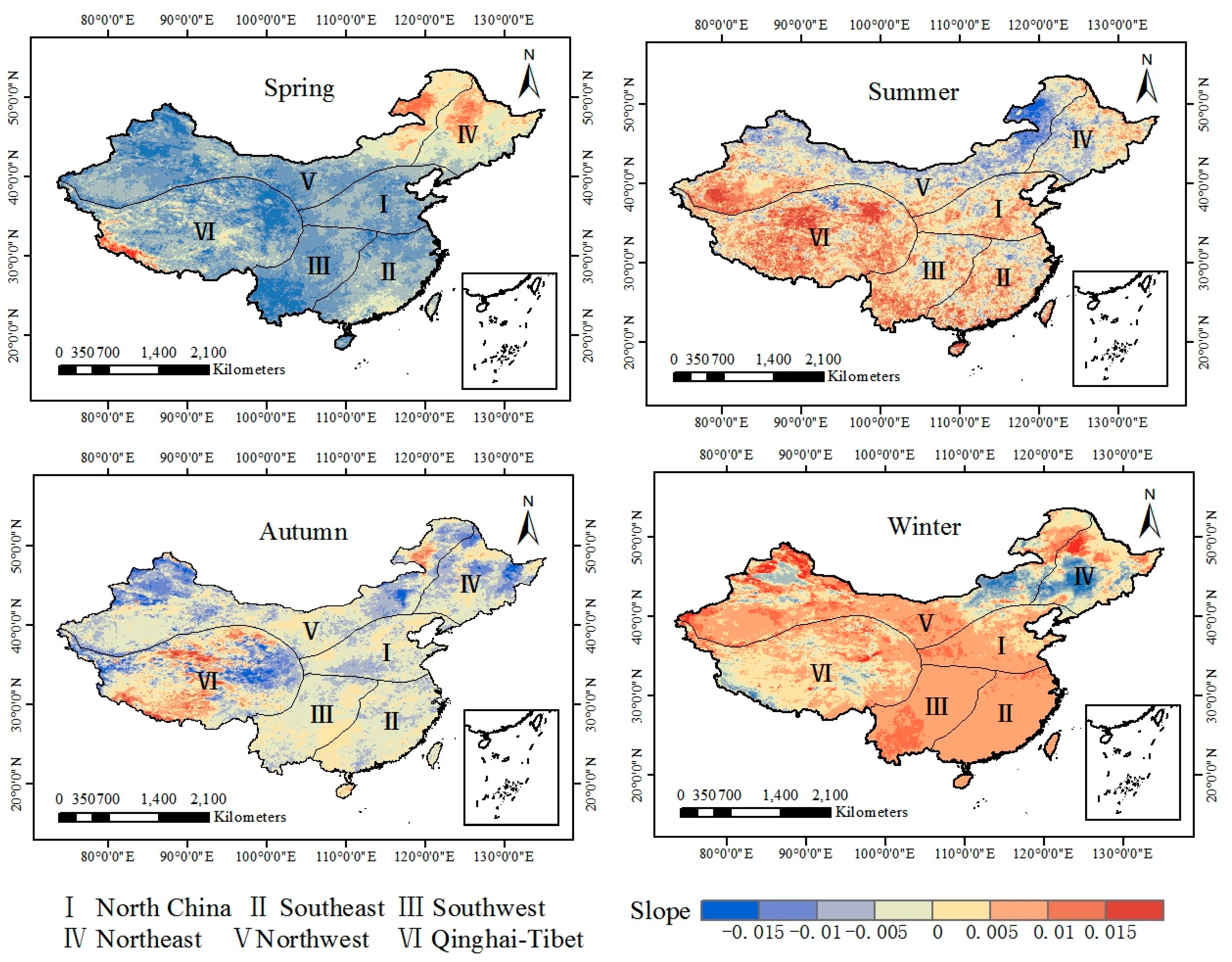
| Very Significantly Decreasing | Significantly Decreasing | Basically Unchanged | Significantly Increasing | Very Significantly Increasing | |
|---|---|---|---|---|---|
| Square (million km2) | 0.49 | 1.26 | 5.69 | 1.89 | 0.256 |
| Percentage (%) | 5.13 | 13.14 | 59.33 | 19.73 | 2.68 |
| Very Significantly Decreasing | Significantly Decreasing | Basically Unchanged | Significantly Increasing | Very Significantly Increasing | ||
|---|---|---|---|---|---|---|
| Spring | Square (million km2) | 2.94 | 4.78 | 1.34 | 0.5 | 3.75 |
| Percentage (%) | 30.69 | 49.77 | 13.97 | 5.19 | 0.39 | |
| Summer | Square (million km2) | 0.42 | 2.2 | 3.28 | 2.72 | 0.97 |
| Percentage (%) | 4.39 | 22.96 | 34.14 | 28.36 | 10.14 | |
| Autumn | Square (million km2) | 0.6 | 3.08 | 5.21 | 0.6 | 10.92 |
| Percentage (%) | 6.21 | 32.08 | 54.35 | 6.22 | 1.14 | |
| Winter | Square (million km2) | 0.31 | 0.73 | 2.09 | 6.19 | 28.81 |
| Percentage (%) | 3.23 | 7.58 | 21.74 | 64.46 | 3.00 |
© 2019 by the authors. Licensee MDPI, Basel, Switzerland. This article is an open access article distributed under the terms and conditions of the Creative Commons Attribution (CC BY) license (http://creativecommons.org/licenses/by/4.0/).
Share and Cite
Tan, J.; NourEldeen, N.; Mao, K.; Shi, J.; Li, Z.; Xu, T.; Yuan, Z. Deep Learning Convolutional Neural Network for the Retrieval of Land Surface Temperature from AMSR2 Data in China. Sensors 2019, 19, 2987. https://doi.org/10.3390/s19132987
Tan J, NourEldeen N, Mao K, Shi J, Li Z, Xu T, Yuan Z. Deep Learning Convolutional Neural Network for the Retrieval of Land Surface Temperature from AMSR2 Data in China. Sensors. 2019; 19(13):2987. https://doi.org/10.3390/s19132987
Chicago/Turabian StyleTan, Jiancan, Nusseiba NourEldeen, Kebiao Mao, Jiancheng Shi, Zhaoliang Li, Tongren Xu, and Zijin Yuan. 2019. "Deep Learning Convolutional Neural Network for the Retrieval of Land Surface Temperature from AMSR2 Data in China" Sensors 19, no. 13: 2987. https://doi.org/10.3390/s19132987
APA StyleTan, J., NourEldeen, N., Mao, K., Shi, J., Li, Z., Xu, T., & Yuan, Z. (2019). Deep Learning Convolutional Neural Network for the Retrieval of Land Surface Temperature from AMSR2 Data in China. Sensors, 19(13), 2987. https://doi.org/10.3390/s19132987