Author Contributions
Conceptualization, M.A.C.-C. and V.A.-R.; Methodology, M.A.C.-C.; Software, M.A.C.-C.; Validation, V.A.-R., U.H.H.-B., and J.P.R.-P.; Investigation, M.A.C.-C.; Resources, J.P.R.-P. and U.H.H.-B.; Data Curation, U.H.H.-B. and J.P.R.-P.; Writing—Original Draft Preparation, M.A.C.-C.; Writing—Review and Editing, M.A.C.-C., V.A.-R., U.H.H.-B., and J.P.R.-P.; Supervision, V.A.-R.
Figure 1.
Graphical description of the proposed system for visual exploration and inspection tasks. SECoS: simple evolving connectionist systems.
Figure 1.
Graphical description of the proposed system for visual exploration and inspection tasks. SECoS: simple evolving connectionist systems.
Figure 2.
Graphical description of the SECoS network. Adaptation of the general ECoS representation from Watts [
29].
Figure 2.
Graphical description of the SECoS network. Adaptation of the general ECoS representation from Watts [
29].
Figure 3.
Graphical representation of the grow-when-required (GWR) neural network. Adaptation of the network architecture presented by Neto et al. [
20].
Figure 3.
Graphical representation of the grow-when-required (GWR) neural network. Adaptation of the network architecture presented by Neto et al. [
20].
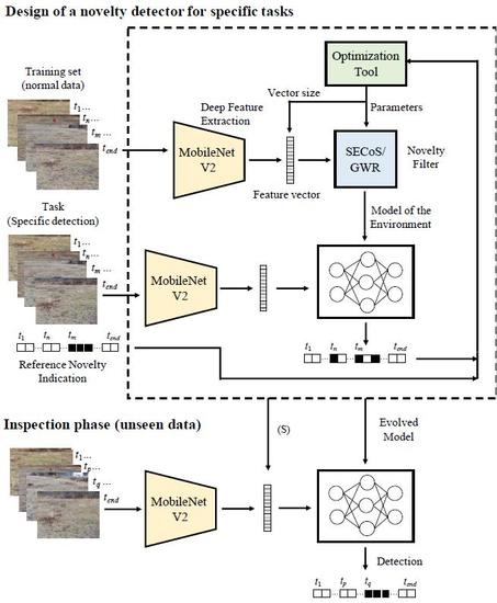
Figure 4.
Flowchart of the visual novelty detection for specific tasks. In the training phase, the novelty filter learns to detect a specific object. In the inspection phase, the evolved model is used to detect the object(s) in the environment.
Figure 4.
Flowchart of the visual novelty detection for specific tasks. In the training phase, the novelty filter learns to detect a specific object. In the inspection phase, the evolved model is used to detect the object(s) in the environment.
Figure 5.
Parrot Bebop 2 Drone with a 14-Mpx flight camera. In the bottom-left corner, we show its visual sensor system.
Figure 5.
Parrot Bebop 2 Drone with a 14-Mpx flight camera. In the bottom-left corner, we show its visual sensor system.
Figure 6.
Experimental setup: the outdoor environment, and some sample captured images. UAV: unmanned aerial vehicle.
Figure 6.
Experimental setup: the outdoor environment, and some sample captured images. UAV: unmanned aerial vehicle.
Figure 7.
Sample images captured by the UAV in the environments: (a) original in the morning (O-1), (b) the person in the morning (O-2), (c) the tire in the morning (O-3), (d) the person and the tire in the morning (O-4), (e) empty environment in the afternoon (O-5), (f) the person in the afternoon (O-6), (g) the boxes in the afternoon (O-7), and (h) the person and the boxes in the afternoon (O-8).
Figure 8.
Average time (seconds) to generate the visual features using different descriptors on all datasets.
Figure 8.
Average time (seconds) to generate the visual features using different descriptors on all datasets.
Figure 9.
Average fitness value of the best-evolved detectors by using the artificial bee colony (ABC) algorithm in the 30 independent runs on dataset D-2. The detectors used the MNF feature extraction technique: (a) GWR detector; (b) SECoS detector.
Figure 9.
Average fitness value of the best-evolved detectors by using the artificial bee colony (ABC) algorithm in the 30 independent runs on dataset D-2. The detectors used the MNF feature extraction technique: (a) GWR detector; (b) SECoS detector.
Figure 10.
Average CPU time (seconds) to generate a specific novelty detector for each dataset by using different feature extraction techniques: (a) GWR detectors; (b) SECoS detectors.
Figure 10.
Average CPU time (seconds) to generate a specific novelty detector for each dataset by using different feature extraction techniques: (a) GWR detectors; (b) SECoS detectors.
Figure 11.
Illustration of the visual exploration and inspection task on dataset D-3 to detect the black tire as the novel object. In the exploration phase, the SECoS detector constructs a model of the environment with the person. In the inspection phase, the detector uses this model to detect the black tire.
Figure 12.
Sample image frames labeled as normal images by the evolved SECoS detector in the inspection phase: (a) sample image frames used to learn the model of the environment, and (b) sample images detected as normal images in the inspection phase.
Figure 12.
Sample image frames labeled as normal images by the evolved SECoS detector in the inspection phase: (a) sample image frames used to learn the model of the environment, and (b) sample images detected as normal images in the inspection phase.
Figure 13.
Sample image frames labeled as novelty images by the evolved SECoS detector in the inspection phase: (a) sample images frames used to learn the model of the environment, and (b) sample images detected as novelty in the inspection phase.
Figure 13.
Sample image frames labeled as novelty images by the evolved SECoS detector in the inspection phase: (a) sample images frames used to learn the model of the environment, and (b) sample images detected as novelty in the inspection phase.
Figure 14.
Visual results in novelty detection on dataset D-1, with the person as the novel object.
Figure 14.
Visual results in novelty detection on dataset D-1, with the person as the novel object.
Figure 15.
Visual results in novelty detection on dataset D-2, with the tire as the novel object.
Figure 15.
Visual results in novelty detection on dataset D-2, with the tire as the novel object.
Figure 16.
Visual results in novelty detection on dataset D-3 (the tire as the novel object, and the person as the normal object).
Figure 16.
Visual results in novelty detection on dataset D-3 (the tire as the novel object, and the person as the normal object).
Figure 17.
Visual results in novelty detection on dataset D-4 (the person as the novel object and the tire as the normal object).
Figure 17.
Visual results in novelty detection on dataset D-4 (the person as the novel object and the tire as the normal object).
Figure 18.
Visual results in novelty detection on dataset D-5, with the person and the tire as the novel objects.
Figure 18.
Visual results in novelty detection on dataset D-5, with the person and the tire as the novel objects.
Figure 19.
Visual results in novelty detection on dataset D-6 (the brown boxes as the novel objects).
Figure 19.
Visual results in novelty detection on dataset D-6 (the brown boxes as the novel objects).
Figure 20.
Visual results in novelty detection on dataset D-7 (the brown boxes as the novel objects).
Figure 20.
Visual results in novelty detection on dataset D-7 (the brown boxes as the novel objects).
Figure 21.
Failure cases in the evolved GWR detector on dataset D-4: (a) sample image frames in the exploration phase, and (b) false novelty indications in the inspection phase. In the exploration phase, the UAV explores environment O-3. Then, it should detect the person as the novelty in environment O-4. In the inspection phase, due to changes in perspective in the frames induced by the UAV’s flight, some false novelty detections were presented because the information of the frame encoding was too different from the learned model.
Table 1.
Parameters to be tuned for each novelty detector.
Table 1.
Parameters to be tuned for each novelty detector.
| Novelty Detector | Parameter | Description |
|---|
| SECoS | | Learning rate 1 |
| | | Learning rate 2 |
| | | Sensitivity threshold |
| | | Error threshold |
| GWR | | Activation threshold |
| | | Habituation threshold |
| | | Proportionality factor |
| | | Learning rate |
Table 2.
Summary of the environments used in the experiments for novelty detection.
Table 2.
Summary of the environments used in the experiments for novelty detection.
| Environment | Description | Loops | #Normal | #Novel |
|---|
| O-1 | Original setup of the environment (morning). | 2 | 896 | 0 |
| O-2 | A person in the O-1 environment (morning). | 2 | 836 | 60 |
| O-3 | Inclusion of a tire to the O-1 environment (morning). | 2 | 838 | 58 |
| O-4 | A person and tire in the O-1 environment (morning). | 2 | 795 | 101 |
| O-5 | Empty environment (afternoon). | 2 | 896 | 0 |
| O-6 | A person in the O-5 environment (afternoon). | 2 | 822 | 74 |
| O-7 | Inclusion of brown boxes to the O-5 environment (afternoon). | 2 | 835 | 61 |
| O-8 | A person and boxes in the O-5 environment (afternoon). | 2 | 825 | 71 |
Table 3.
Data partition for novelty detection.
Table 3.
Data partition for novelty detection.
| Dataset | Exploration | Inspection | Test Case (Novelty) |
|---|
| D-1 | O-1 | O-2 | A dynamic object (person). |
| D-2 | O-1 | O-3 | A small conspicuous object (black tire). |
| D-3 | O-2 | O-4 | A conspicuous object in a dynamic environment (black tire). |
| D-4 | O-3 | O-4 | A dynamic object in an environment with a conspicuous object (person). |
| D-5 | O-1 | O-4 | Multiple novel objects (person and tire). |
| D-6 | O-5 | O-7 | Inconspicuous objects (brown boxes). |
| D-7 | O-6 | O-8 | Occlusion of inconspicuous objects (brown boxes). |
Table 4.
Confusion matrix to evaluate the performance of the novelty detectors. : false negative; : false positive; : true negative; : true positive.
Table 4.
Confusion matrix to evaluate the performance of the novelty detectors. : false negative; : false positive; : true negative; : true positive.
| Class/Prediction | Normal | Novel |
|---|
| Normal | | |
| Novel | | |
Table 5.
Average results in the inspection phase over the 30 runs. Bold values indicate the best result for each metric according to the specific dataset and the specific novelty detector. CAI: color angular indexing; hRGB: RGB color histogram; MNF: feature extraction based on MobileNetV2; : average vector size; : average model size; : true positive rate; : true negative rate; : score; : accuracy; : Matthews correlation coefficient; R: ranking of the detector.
| Dataset | Detector | Descriptor | VSize | MSize | | | | ACC | MCC | R |
|---|
| D-1 | SECoS | CAI | 4.0 | 17.5 | 0.9692 | 0.2750 | 0.9607 | 0.9258 | 0.2865 | 4.0 |
| hRGB | 305.0 | 12.4 | 0.9738 | 0.4571 | 0.9689 | 0.9415 | 0.4673 | 3.0 |
| GIST | 350.5 | 47.5 | 0.9867 | 0.8571 | 0.9886 | 0.9786 | 0.8312 | 2.0 |
| MNF | 169.1 | 7.1 | 0.9922 | 0.9000 | 0.9928 | 0.9865 | 0.8859 | 1.0 |
| GWR | CAI | 4.0 | 29.1 | 0.9520 | 0.3238 | 0.9532 | 0.9127 | 0.2530 | 3.6 |
| hRGB | 357.3 | 20.5 | 0.9757 | 0.2393 | 0.9628 | 0.9297 | 0.2317 | 3.4 |
| GIST | 398.1 | 46.7 | 0.9900 | 0.8452 | 0.9898 | 0.9810 | 0.8418 | 1.8 |
| MNF | 153.3 | 13.8 | 0.9899 | 0.8869 | 0.9912 | 0.9835 | 0.8646 | 1.2 |
| D-2 | SECoS | CAI | 4.0 | 13.6 | 0.9879 | 0.0155 | 0.9620 | 0.9271 | 0.0076 | 2.6 |
| hRGB | 337.0 | 25.3 | 0.9734 | 0.0857 | 0.9567 | 0.9179 | 0.0655 | 3.0 |
| GIST | 384.9 | 37.7 | 0.8444 | 0.8333 | 0.9084 | 0.8438 | 0.4295 | 3.2 |
| MNF | 143.3 | 16.6 | 0.9806 | 0.9976 | 0.9901 | 0.9817 | 0.8729 | 1.2 |
| GWR | CAI | 4.0 | 2.4 | 0.9943 | 0.0000 | 0.9649 | 0.9321 | −0.0104 | 3.0 |
| hRGB | 365.4 | 2.0 | 1.0000 | 0.0000 | 0.9677 | 0.9375 | 0.0000 | 2.2 |
| GIST | 334.3 | 79.8 | 0.8300 | 0.7821 | 0.8976 | 0.8270 | 0.3758 | 3.2 |
| MNF | 180.8 | 23.7 | 0.9852 | 0.9548 | 0.9910 | 0.9833 | 0.8729 | 1.4 |
| D-3 | SECoS | CAI | 4.0 | 11.8 | 0.9426 | 0.6086 | 0.9561 | 0.9195 | 0.4765 | 2.2 |
| hRGB | 427.2 | 29.3 | 0.9642 | 0.1452 | 0.9507 | 0.9075 | 0.0914 | 3.2 |
| GIST | 269.0 | 50.2 | 0.9019 | 0.6022 | 0.9323 | 0.8812 | 0.3742 | 3.6 |
| MNF | 184.1 | 27.8 | 0.9788 | 0.8484 | 0.9836 | 0.9698 | 0.7881 | 1.0 |
| GWR | CAI | 4.0 | 6.5 | 0.9905 | 0.1118 | 0.9632 | 0.9297 | 0.1111 | 2.4 |
| hRGB | 445.0 | 6.1 | 0.9922 | 0.0118 | 0.9602 | 0.9244 | 0.0024 | 3.0 |
| GIST | 353.4 | 152.2 | 0.9117 | 0.4645 | 0.9317 | 0.8807 | 0.2852 | 3.2 |
| MNF | 216.0 | 34.2 | 0.9723 | 0.8710 | 0.9812 | 0.9653 | 0.7653 | 1.4 |
| D-4 | SECoS | CAI | 4.0 | 16.9 | 0.9790 | 0.0157 | 0.9703 | 0.9424 | −0.0072 | 3.6 |
| hRGB | 303.2 | 29.5 | 0.9745 | 0.3000 | 0.9733 | 0.9489 | 0.3008 | 3.0 |
| GIST | 315.0 | 2.2 | 0.9912 | 0.8706 | 0.9930 | 0.9866 | 0.8259 | 1.0 |
| MNF | 147.2 | 15.8 | 0.9729 | 0.8098 | 0.9825 | 0.9667 | 0.6585 | 2.4 |
| GWR | CAI | 4.0 | 6.1 | 0.9947 | 0.0000 | 0.9780 | 0.9570 | −0.0105 | 3.0 |
| hRGB | 289.0 | 51.9 | 0.9552 | 0.3176 | 0.9633 | 0.9310 | 0.2046 | 3.6 |
| GIST | 334.0 | 15.3 | 0.9690 | 0.9039 | 0.9821 | 0.9665 | 0.7279 | 1.8 |
| MNF | 173.8 | 15.4 | 0.9770 | 0.7784 | 0.9840 | 0.9695 | 0.6578 | 1.6 |
| D-5 | SECoS | CAI | 4.0 | 7.5 | 0.9765 | 0.0778 | 0.9356 | 0.8802 | 0.0945 | 3.8 |
| hRGB | 276.5 | 40.4 | 0.9823 | 0.1299 | 0.9414 | 0.8910 | 0.1976 | 2.6 |
| GIST | 306.7 | 24.6 | 0.9536 | 0.5764 | 0.9512 | 0.9132 | 0.5516 | 2.4 |
| MNF | 180.0 | 26.9 | 0.9813 | 0.9472 | 0.9874 | 0.9776 | 0.8916 | 1.2 |
| GWR | CAI | 4.0 | 7.8 | 0.9749 | 0.1049 | 0.9361 | 0.8817 | 0.1565 | 3.2 |
| hRGB | 331.4 | 36.6 | 0.9833 | 0.0660 | 0.8978 | 0.8850 | 0.0795 | 3.4 |
| GIST | 385.9 | 46.7 | 0.9305 | 0.6403 | 0.9420 | 0.8994 | 0.5475 | 2.4 |
| MNF | 221.8 | 26.9 | 0.9917 | 0.8681 | 0.9880 | 0.9784 | 0.8847 | 1.0 |
| D-6 | SECoS | CAI | 4.0 | 7.9 | 0.9560 | 0.0344 | 0.9439 | 0.8943 | −0.0206 | 3.2 |
| hRGB | 213.2 | 6.0 | 0.9270 | 0.8900 | 0.9580 | 0.9246 | 0.6233 | 2.4 |
| GIST | 245.4 | 9.5 | 0.8352 | 0.9167 | 0.9059 | 0.8407 | 0.4707 | 3.2 |
| MNF | 150.2 | 20.4 | 0.9750 | 0.8911 | 0.9834 | 0.9693 | 0.7950 | 1.2 |
| GWR | CAI | 4.0 | 11.6 | 0.9761 | 0.0200 | 0.9535 | 0.9121 | −0.0045 | 2.8 |
| hRGB | 304.3 | 61.3 | 0.8946 | 0.8622 | 0.9388 | 0.8924 | 0.5277 | 2.8 |
| GIST | 289.0 | 11.5 | 0.7977 | 0.9111 | 0.8825 | 0.8053 | 0.4194 | 3.2 |
| MNF | 210.5 | 16.0 | 0.9796 | 0.8878 | 0.9857 | 0.9734 | 0.8107 | 1.2 |
| D-7 | SECoS | CAI | 4.0 | 8.5 | 0.9730 | 0.0192 | 0.9487 | 0.9028 | −0.0085 | 3.8 |
| hRGB | 276.6 | 6.3 | 0.9482 | 0.9939 | 0.9731 | 0.9516 | 0.7605 | 2.8 |
| GIST | 444.9 | 9.9 | 0.9867 | 0.9364 | 0.9907 | 0.9829 | 0.8831 | 2.0 |
| MNF | 165.2 | 17.6 | 0.9855 | 0.9848 | 0.9921 | 0.9855 | 0.9065 | 1.4 |
| GWR | CAI | 4.0 | 2.8 | 0.9982 | 0.0000 | 0.9609 | 0.9247 | −0.0021 | 3.2 |
| hRGB | 255.7 | 12.2 | 0.9369 | 0.8424 | 0.9607 | 0.9300 | 0.6307 | 3.4 |
| GIST | 370.7 | 14.4 | 0.9654 | 0.9030 | 0.9783 | 0.9608 | 0.7757 | 2.2 |
| MNF | 175.7 | 8.1 | 0.9862 | 0.9960 | 0.9929 | 0.9869 | 0.9162 | 1.2 |
Table 6.
Set of sample evolved detectors generated by the proposed global optimization framework on all the datasets.
Table 6.
Set of sample evolved detectors generated by the proposed global optimization framework on all the datasets.
| Detector | Dataset | | | | | VSize |
|---|
| SECoS | D-1 | 0.2002440 | 0.2428720 | 0.0545579 | 0.4578700 | 170 |
| D-2 | 0.2045570 | 0.2697980 | 0.5078360 | 0.2089900 | 74 |
| D-3 | 0.0183574 | 0.4830270 | 0.4651190 | 0.7776980 | 256 |
| D-4 | 0.1456960 | 0.3827950 | 0.1083890 | 0.2627370 | 75 |
| D-5 | 0.0000000 | 0.0109682 | 0.2810780 | 0.5950580 | 242 |
| D-6 | 0.0000000 | 0.0000000 | 0.6285940 | 0.5863690 | 144 |
| D-7 | 0.6577200 | 0.2922090 | 0.1750940 | 0.4164290 | 96 |
| | | | | | | VSize |
| GWR | D-1 | 0.6827340 | 0.6826510 | 0.0706664 | 0.0490785 | 152 |
| D-2 | 0.7888710 | 0.2963600 | 0.3931710 | 0.0000000 | 101 |
| D-3 | 0.5653500 | 0.3496060 | 0.4179080 | 0.0631437 | 249 |
| D-4 | 0.5521850 | 0.4037900 | 0.2024040 | 0.0000000 | 216 |
| D-5 | 0.5756130 | 0.8404430 | 0.0000000 | 0.0000000 | 256 |
| D-6 | 0.7806360 | 0.7388830 | 0.2143130 | 0.0000000 | 67 |
| D-7 | 0.5295850 | 0.6676220 | 0.0790152 | 0.7237070 | 135 |
Table 7.
Results in the inspection phase (unseen data) of the sample evolved detectors. Bold values indicate the best result for each metric.
Table 7.
Results in the inspection phase (unseen data) of the sample evolved detectors. Bold values indicate the best result for each metric.
| Dataset | Detector | MSize | | | | ACC | MCC |
|---|
| D-1 | SECoS | 6 | 0.9976 | 0.9643 | 0.9976 | 0.9955 | 0.9619 |
| GWR | 9 | 0.9952 | 0.9643 | 0.9964 | 0.9933 | 0.9440 |
| D-2 | SECoS | 12 | 0.9929 | 1.0000 | 0.9964 | 0.9933 | 0.9470 |
| GWR | 27 | 0.9929 | 1.0000 | 0.9964 | 0.9933 | 0.9470 |
| D-3 | SECoS | 18 | 0.9976 | 0.9677 | 0.9976 | 0.9955 | 0.9653 |
| GWR | 21 | 0.9856 | 0.9677 | 0.9915 | 0.9843 | 0.8900 |
| D-4 | SECoS | 11 | 0.9930 | 0.7647 | 0.9919 | 0.9844 | 0.7802 |
| GWR | 19 | 0.9861 | 0.7647 | 0.9884 | 0.9777 | 0.7118 |
| D-5 | SECoS | 23 | 0.9975 | 0.9792 | 0.9975 | 0.9955 | 0.9767 |
| GWR | 32 | 0.9975 | 0.9375 | 0.9950 | 0.9911 | 0.9527 |
| D-6 | SECoS | 17 | 0.9952 | 0.9000 | 0.9940 | 0.9888 | 0.9094 |
| GWR | 14 | 0.9904 | 0.9000 | 0.9916 | 0.9844 | 0.8770 |
| D-7 | SECoS | 9 | 0.9952 | 1.0000 | 0.9976 | 0.9955 | 0.9687 |
| GWR | 4 | 0.9928 | 1.0000 | 0.9964 | 0.9933 | 0.9540 |

 ,
, 


