A Novel Deep-Learning-Based Bug Severity Classification Technique Using Convolutional Neural Networks and Random Forest with Boosting


Abstract

1. Introduction
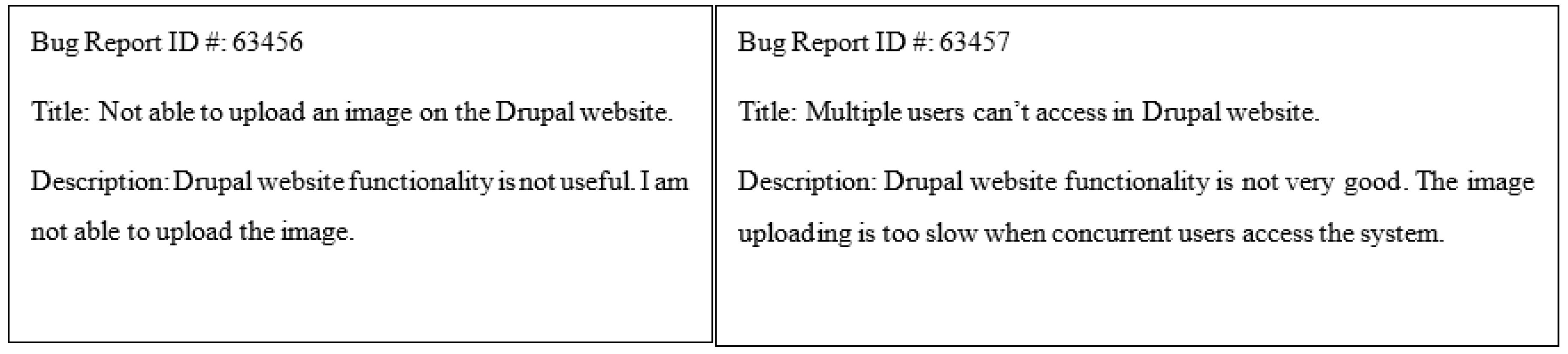
1.1. Motivation Example
1.2. Research Contribution
- Whether it is feasible to implement automated multi-bug severity classification model using deep learning technique and what the best configuration of Bug Severity classification is via Convolutional Neural Network and Random forest (BCR);
- Whether the proposed algorithm outperforms the Traditional machine learning algorithms in bug severity classification.
- To the best of our knowledge, we have taken the first step to build the multiclass bug severity classification model via deep learning and random forest for open source projects;
- The n-gram technique is employed to generate the features from the text, which captures word order and the characteristics of different severity classes in five open source projects;
- A CNN-based feature representation framework is proposed to automatically generate the semantic and non-linear mapping of features, which preserves the semantic information of the bug report text;
- The CNN and random forest with boosting acclimates for severity classification instead of the traditional machine learning algorithms. The evaluation results show that the proposed algorithm outperforms the other algorithms in binary and multiple bug severity classification.
2. Related Work
2.1. Binary Classification
2.2. Multiclass Classification
3. Research Methodology
3.1. Overall Framework
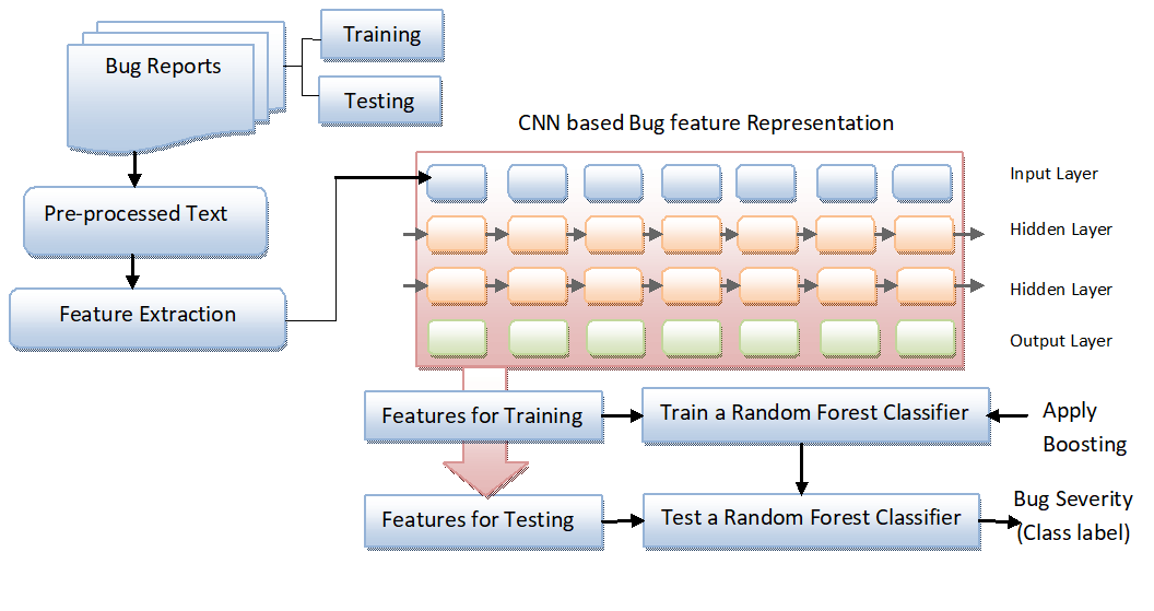
- The bug reports with a title, description, and summary are considered for the input, and the code snippets, URLs, hexcode, and stacktraces of the bug report are removed;
- As seen in Figure 4, the initial step is preprocessing; in this, each word of the bug report content is converted into more manageable representation (Section 3.2). The preprocessed content goes through the next step, which is n-gram Extraction (NE). In the NE step, a set of n-gram features (words) are extracted, which enlarges the word integer into the Feature and Label matrix, which illustrates them in a meaningful way (Section 3.3). The output of NE goes into the Feature Extraction with Convolutional Neural Network (FECNN). It learns semantically meaningful representations of the sentences. It is consists of seven hidden layers. Each hidden layer contains a convolutional layer, max pooling layer, activation function, dropout layer, and fully connected layer. Firstly, the features are extracted by the CNN in the convolutional layer (CL), which extracts and transforms the features by max pooling (PL). Further, the fully connected layer (FL) combines all the features to develop feature space (Section 3.4). Dropout layers and activation functions are utilized before and after the convolutional layer. In the first three layers, the sigmoid activation function is used, and in the last tanh, the activation function is used. It gives the output as a feature vector, and these are fed into the classification layer (CLL), which is utilized to classify the severity of each bug report (Section 3.5). Section 3.5 is divided into three further sections. The initial Section 3.5.1 explains the full process of feature extraction via CNN and random forest with boosting classifier (CNRFB). Section 3.5.2 and Section 3.5.3 illustrate the training process of CNRFB and the process of random forest with boosting classifier (RFB).
- The bug report dataset is divided into training and testing with 10-fold cross-validation to avoid the training biases. The supervised classifier is trained with the features that are extracted by the FECNN module in the training part. In the testing part, the extracted features are used by the trained classifier for severity classification.
3.2. Preprocessing
3.3. N-Gram Extraction
3.4. Feature Extraction with Convolutional Neural Network (FECNN)
3.5. FECNN with Random Forest with Boosting Classifier (CNRFB)
3.5.1. CNRFB Model
3.5.2. Training Procedure of CNRFB
| Algorithm 1: The Training Process of CNR Model |
| Input: Training Bug Report Dataset BRD= ; Maximum Iteration:MI; Threshold:; Batch Size: BS; Iteration Time: IT Output: CNRFB model cnrfb_model |
|
3.5.3. Random Forest with Boosting Classifier (RFB)
4. Experimental Setup
4.1. Dataset
4.2. Parameter Settings
5. Results
6. Threats to Validity
- The results are manifested using five bug repositories with distinct characteristics to assure generalization. Further, commercial BTS may accompany different patterns, and hence the BCR model outcomes may not be legitimately extensible to such bug repositories;
- Currently, in the BCR model, only the descriptions and titles of bug reports are examined. While these two-unstructured data are significant, as shown by the experiments, there exists other structured data that are required to classify the bug severity sufficiently;
- Generally, most of the bug reports are misclassified. Therefore, the experiment is conducted on manually labeled bug datasets from the actual paper. Although the actual paper proposes some rule sets to support their severity classification, errors might occur. These rules and labeling process depend on a personal perspective;
- Assuring that the statistical methods are reliable is yet another challenge. From this, the collinear variables are removed to confirm that the bug report data is not inflated. The statistical tests are applied, and the bug report dataset is adjusted by using stratified sampling;
- The other step is to assure that the BCR model does not experience overfitting, therefore the K-fold-cross-validation is applied, where each sample is used for both training and testing, thus providing a more accurate model.
7. Conclusions
Author Contributions
Funding
Conflicts of Interest
References
- Sharma, Y.; Dagur, A.; Chaturvedi, R. Automated bug reporting system with keyword-driven framework. In Soft Computing and Signal Processing; Springer: Singapore, 2019; pp. 271–277. [Google Scholar]
- Canfora, G.; Cerulo, L. How software repositories can help in resolving a new change request. In Proceedings of the 13th IEEE International Workshop on Software Technology and Engineering Practice, Budapest, Hungary, 24–25 September 2005; pp. 89–99. [Google Scholar]
- Antoniol, G.; Ayari, K.; Di Penta, M.; Khomh, F.; Guéhéneuc, Y.G. Is it a bug or an enhancement?: a text-based approach to classify change requests. In Proceedings of the ACM 2008 Conference of the Center for Advanced Studies on Collaborative Research: Meeting of Minds, Ontario, Canada, 27–30 October 2008; p. 23. [Google Scholar]
- Angel, T.S.; Kumar, G.S.; Sehgal, V.M.; Nayak, G. Effective bug processing and tracking system. J. Comput. Theor. Nanosci. 2018, 15, 2604–2606. [Google Scholar] [CrossRef]
- Nagwani, N.K.; Verma, S.; Mehta, K.K. Generating taxonomic terms for software bug classification by utilizing topic models based on Latent Dirichlet Allocation. In Proceedings of the IEEE 11th International Conference on ICT and Knowledge Engineering (ICT&KE), Bangkok, Thailand, 20–22 November 2013; pp. 1–5. [Google Scholar]
- Guo, S.; Chen, R.; Wei, M.; Li, H.; Liu, Y. Ensemble data reduction techniques and Multi-RSMOTE via fuzzy integral for bug report classification. IEEE Access 2018, 6, 45934–45950. [Google Scholar] [CrossRef]
- Catal, C.; Diri, B. A systematic review of software fault prediction studies. Exp. Syst. Appl. 2009, 36, 7346–7354. [Google Scholar] [CrossRef]
- Chaturvedi, K.K.; Singh, V.B. Determining bug severity using machine learning techniques. In Proceedings of the Software Engineering (CONSEG), Sixth International Conference on CSI, Indore, India, 5–7 September 2012; pp. 1–6. [Google Scholar]
- Gegick, M.; Rotella, P.; Xie, T. Identifying security bug reports via text mining: An industrial case study. In Proceedings of the 7th IEEE Working Conference on Mining Software Repositories (MSR), Cape Town, South Africa, 2–3 May 2010; pp. 11–20. [Google Scholar]
- Malhotra, R. A systematic review of machine learning techniques for software fault prediction. Appl. Soft Comput. 2015, 27, 504–518. [Google Scholar] [CrossRef]
- Menzies, T.; Marcus, A. Automated severity assessment of software defect reports. In Proceedings of the IEEE International Conference on Software Maintenance, Beijing, China, 28 September–4 October 2008; pp. 346–355. [Google Scholar]
- Chawla, I.; Singh, S.K. An automated approach for bug categorization using fuzzy logic. In Proceedings of the 8th India Software Engineering Conference, Bangalore, India, 18–20 February 2015; pp. 90–99. [Google Scholar]
- Gujral, S.; Sharma, G.; Sharma, S. Classifying bug severity using dictionary based approach. In Proceedings of the International Conference on Futuristic Trends on Computational Analysis and Knowledge Management (ABLAZE), Noida, India, 25–27 February 2015; pp. 599–602. [Google Scholar]
- Pandey, N.; Sanyal, D.K.; Hudait, A.; Sen, A. Automated classification of software issue reports using machine learning techniques: An empirical study. Innov. Syst. Softw. Eng. 2017, 13, 279–297. [Google Scholar] [CrossRef]
- Yang, X.; Huang, K.; Zhang, R.; Hussain, A. Learning latent features with infinite nonnegative binary matrix trifactorization. IEEE Trans. Emerg. Topics Comput. Intell. 2018, 2, 1–14. [Google Scholar] [CrossRef]
- Wei, Y.; Zhao, Y.; Lu, C.; Wei, S.; Liu, L.; Zhu, Z.; Yan, S. Cross-modal retrieval with CNN visual features: A new baseline. IEEE Trans. Cybernet. 2017, 47, 449–460. [Google Scholar] [CrossRef]
- Bengio, Y. Learning deep architectures for A.I. Found. Trends Mach. Learn. 2009, 2, 1–127. [Google Scholar] [CrossRef]
- Dong, F.; Wang, J.; Li, Q.; Xu, G.; Zhang, S. Defect prediction in android binary executables using deep neural network. Wirel. Pers. Commun. 2018, 102, 2261–2285. [Google Scholar] [CrossRef]
- Shi, H.; Xu, M.; Li, R. Deep learning for household load forecasting—A novel pooling deep RNN. IEEE Trans. Smart Grid 2018, 9, 5271–5280. [Google Scholar] [CrossRef]
- Zhang, S.; Zhang, S.; Huang, T.; Gao, W. Speech emotion recognition using deep convolutionalal neural network and discriminant temporal pyramid matching. IEEE Trans. Multim. 2018, 20, 1576–1590. [Google Scholar] [CrossRef]
- Palaz, D.; Magimai-Doss, M.; Collobert, R. End-to-end acoustic modeling using convolutionalal neural networks for HMM-based automatic speech recognition. Speech Commun. 2019, 108, 15–32. [Google Scholar] [CrossRef]
- Han, D.; Liu, Q.; Fan, W. A new image classification method using CNN transfer learning and web data augmentation. Exp. Syst. Appl. 2018, 95, 43–56. [Google Scholar] [CrossRef]
- Wei, Y.; Xia, W.; Lin, M.; Huang, J.; Ni, B.; Dong, J.; Zhao, Y.; Yan, S. HCP: A flexible CNN framework for multi-label image classification. IEEE Trans. Pattern Anal. Mach. Intell. 2016, 38, 1901–1907. [Google Scholar] [CrossRef] [PubMed]
- Zhang, M.; Li, W.; Du, Q. Diverse region-based CNN for hyperspectral image classification. IEEE Trans. Image Process. 2018, 27, 2623–2634. [Google Scholar] [CrossRef] [PubMed]
- Chen, T.; Xu, R.; He, Y.; Wang, X. Improving sentiment analysis via sentence type classification using BiLSTM-CRF and CNN. Exp. Syst. Appl. 2017, 72, 221–230. [Google Scholar] [CrossRef]
- Zhou, Y.; Tong, Y.; Gu, R.; Gall, H. Combining text mining and data mining for bug report classification. J. Softw. Evol. Process 2016, 28, 150–176. [Google Scholar] [CrossRef]
- Jin, K.; Dashbalbar, A.; Yang, G.; Lee, J.-W.; Lee, B. Bug severity prediction by classifying normal bugs with text and meta-field information. Adv. Sci. Technol. Lett. 2016, 129, 19–24. [Google Scholar]
- Lamkanfi, A.; Demeyer, S.; Giger, E.; Goethals, B. Predicting the severity of a reported bug. In Proceedings of the 7th IEEE Working Conference on Mining Software Repositories (MSR), Cape Town, South Africa, 2–3 May 2010; pp. 1–10. [Google Scholar]
- Goseva-Popstojanova, K.; Tyo, J. Identification of security related bug reports via text mining using supervised and unsupervised classification. In Proceedings of the IEEE International Conference on Software Quality, Reliability and Security, Lisbon, Portugal, 16–20 July 2018; pp. 344–355. [Google Scholar]
- Kukkar, A.; Mohana, R. A Supervised bug report classification with incorporate and textual field knowledge. Procedia Comp. Sci. 2018, 132, 352–361. [Google Scholar] [CrossRef]
- Jindal, R.; Malhotra, R.; Jain, A. Prediction of defect severity by mining software project reports. Int. J. Syst. Assur. Eng. Manag. 2017, 8, 334–351. [Google Scholar] [CrossRef]
- Singh, V.B.; Misra, S.; Sharma, M. Bug severity assessment in cross project context and identifying training candidates. J. Inf. Knowl. Manag 2017, 16, 1750005. [Google Scholar] [CrossRef]
- Zhang, T.; Chen, J.; Yang, G.; Lee, B.; Luo, X. Towards more accurate severity prediction and fixer recommendation of software bugs. J. Syst. Softw. 2016, 117, 166–184. [Google Scholar] [CrossRef]
- Sharmin, S.; Aktar, F.; Ali, A.A.; Khan, M.A.H.; Shoyaib, M. BFSp: A feature selection method for bug severity classification. In Proceedings of the Humanitarian Technology Conference (R10-HTC), Dhaka, Bangladesh, 21–23 December 2017; pp. 750–754. [Google Scholar]
- Kumari, M.; Sharma, M.; Singh, V.B. Severity assessment of a reported bug by considering its uncertainty and irregular state. Int. J. Open Source Softw. Process. 2018, 9, 20–46. [Google Scholar] [CrossRef]
- Liang, J.; Koperski, K.; Dhillon, N.S.; Tusk, C.; Bhatti, S. VCVC III LLC. NLP-Based Entity Recognition and Disambiguation. U.S. Patent 8,594,996, 26 November 2013. [Google Scholar]
- Wang, R.; Zhao, H.; Lu, B.L.; Utiyama, M.; Sumita, E. Bilingual continuous-space language model growing for statistical machine translation. IEEE/ACM Trans. Audio Speech Lang. Process. 2015, 23, 1209–1220. [Google Scholar] [CrossRef]
- Zhu, X.; Du, X.; Kerich, M.; Lohoff, F.W.; Momenan, R. Random forest based classification of alcohol dependence patients and healthy controls using resting state MRI. Neurosci. Lett. 2018, 676, 27–33. [Google Scholar] [CrossRef] [PubMed]
- Xia, X.; Togneri, R.; Sohel, F.; Huang, D. Random forest classification based acoustic event detection utilizing contextual-information and bottleneck features. Pattern Recogn. 2018, 81, 1–13. [Google Scholar] [CrossRef]
- Gupta, B.; Awasthi, S.; Gupta, R.; Ram, L.; Kumar, P.; Prasad, B.R.; Agarwal, S. Taxi travel time prediction using ensemble-based random forest and gradient boosting model. In Advances in Big Data and Cloud Computing; Springer: Singapore, 2018; pp. 63–78. [Google Scholar]
- Huang, Y.J.; Powers, R.; Montelione, G.T. Protein NMR recall, precision, and F-measure scores (RPF scores): Structure quality assessment measures based on information retrieval statistics. J. Am. Chem. Soc. 2005, 127, 1665–1674. [Google Scholar] [CrossRef] [PubMed]


| Projects | Number of Bugs | BTS | Number of Classes | Name of Severity Classes |
|---|---|---|---|---|
| Mozilla | 539 | Bugzilla | 7 | Blocker, Critical, Enhancement, Major, Normal, Minor, Trivial |
| Eclipse | 693 | Bugzilla | 5 | Blocker, Critical, Enhancement, Major, Normal |
| JBoss | 573 | RedhatBugzilla | 5 | High, Low, Medium, Unspecified, Urgent |
| OpenFOAM | 795 | Manits | 8 | Blocker, Crash, Feature, Major, Minor, Text, Trivial, Tweak |
| Firefox | 620 | Bugzilla | 7 | Blocker, Critical, Enhancement, Major, Normal, Minor, Trivial |
| Projects | Classes | Precision (%) | Recall (%) | F-Measure (%) | Accuracy (%) |
|---|---|---|---|---|---|
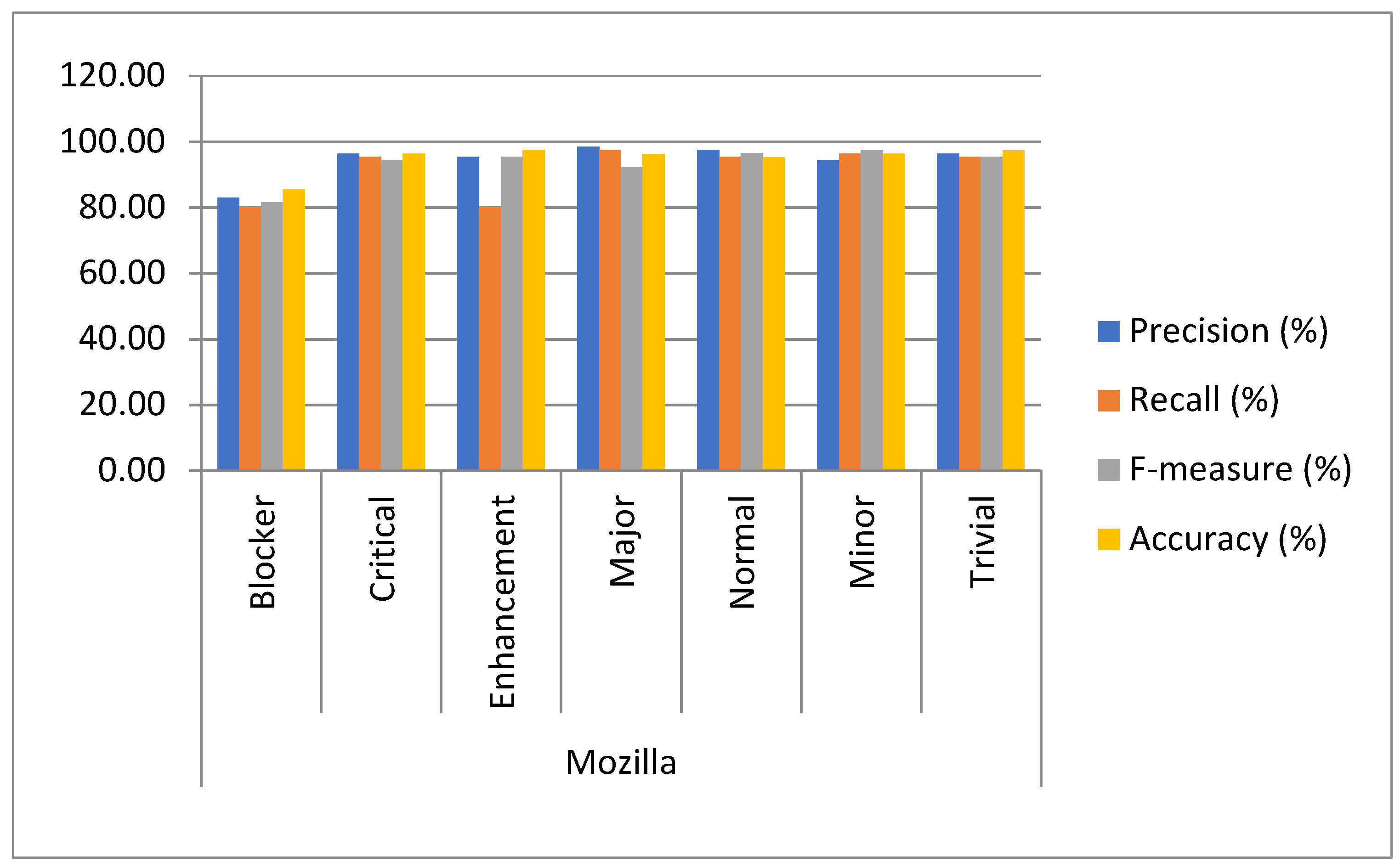
| Mozilla | Blocker | 82.90 | 80.23 | 81.54 | 85.45 |
| Critical | 96.43 | 95.34 | 94.34 | 96.33 | |
| Enhancement | 95.33 | 80.22 | 95.45 | 97.43 | |
| Major | 98.45 | 97.45 | 92.34 | 96.30 | |
| Normal | 97.44 | 95.34 | 96.45 | 95.24 | |
| Minor | 94.35 | 96.34 | 97.44 | 96.34 | |
| Trivial | 96.35 | 95.34 | 95.33 | 97.33 | |
| Firefox | Blocker | 86.16 | 83.35 | 84.73 | 83.00 |
| Critical | 97.97 | 92.23 | 95.27 | 97.92 | |
| Enhancement | 98.30 | 92.23 | 95.98 | 97.55 | |
| Major | 97.98 | 97.61 | 96.64 | 97.19 | |
| Normal | 97.28 | 96.90 | 97.64 | 97.53 | |
| Minor | 97.23 | 97.04 | 97.24 | 98.33 | |
| Trivial | 98.43 | 95.68 | 96.52 | 98.85 | |
| Eclipse | Blocker | 80.34 | 81.23 | 83.45 | 83.45 |
| Critical | 97.33 | 89.23 | 96.35 | 98.33 | |
| Enhancement | 98.34 | 90.29 | 95.35 | 98.32 | |
| Major | 99.40 | 97.85 | 95.85 | 97.22 | |
| Normal | 97.35 | 97.29 | 98.40 | 97.24 | |
| Jboss | High | 96.80 | 97.29 | 97.84 | 98.29 |
| Low | 98.27 | 97.00 | 96.75 | 98.93 | |
| Medium | 99.08 | 95.45 | 96.72 | 99.22 | |
| Unspecified | 99.59 | 93.68 | 97.08 | 99.19 | |
| Urgent | 99.59 | 96.37 | 97.76 | 98.82 | |
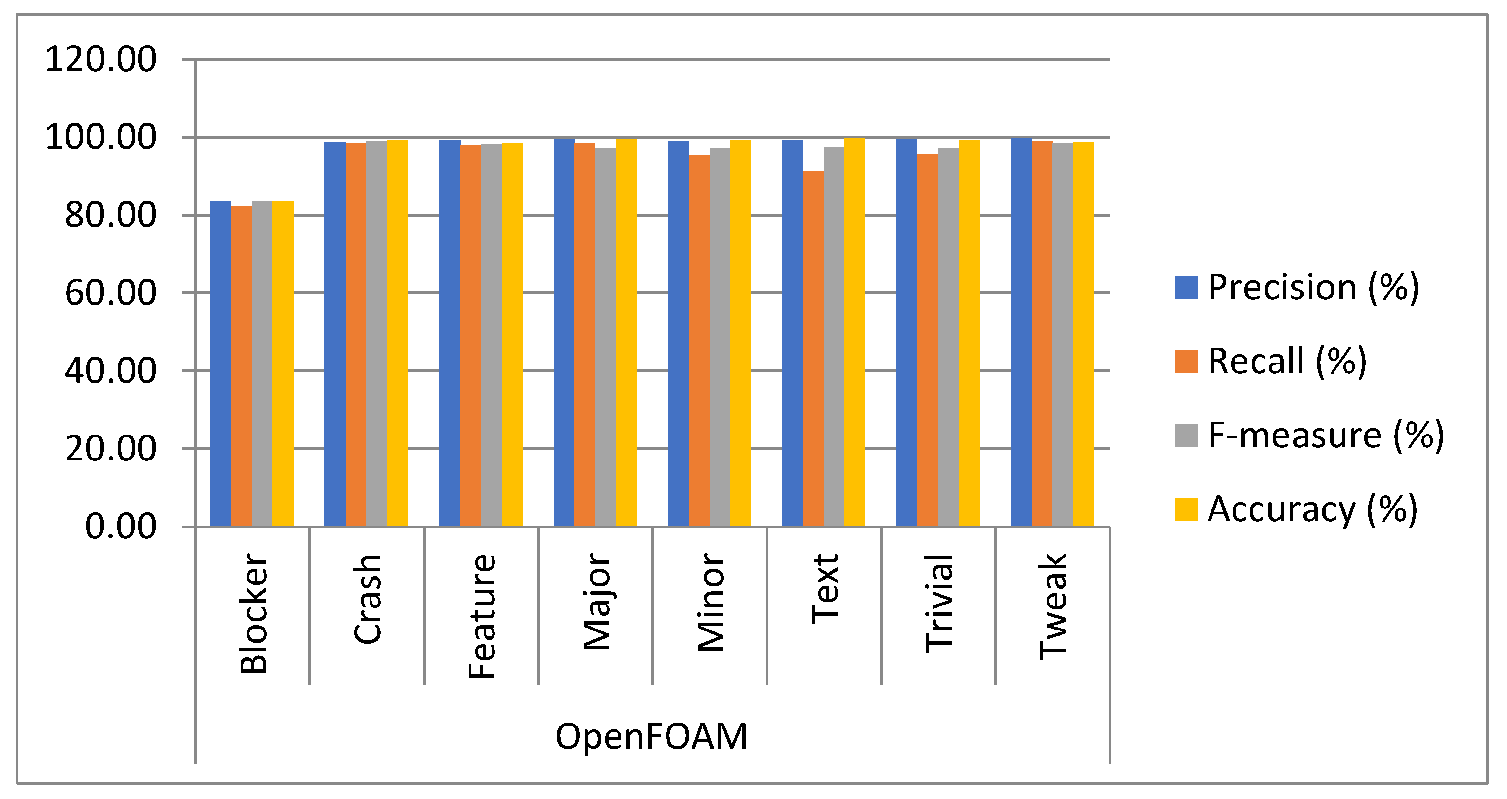
| OpenFOAM | Blocker | 83.45 | 82.34 | 83.45 | 83.40 |
| Crash | 98.70 | 98.42 | 98.89 | 99.38 | |
| Feature | 99.28 | 97.81 | 98.33 | 98.56 | |
| Major | 99.61 | 98.51 | 97.11 | 99.54 | |
| Minor | 99.06 | 95.29 | 97.02 | 99.28 | |
| Text | 99.29 | 91.21 | 97.30 | 99.77 | |
| Trivial | 99.45 | 95.52 | 97.05 | 99.22 | |
| Tweak | 99.82 | 99.02 | 98.57 | 98.68 |
| Approach | Result Analysis | ||||
|---|---|---|---|---|---|
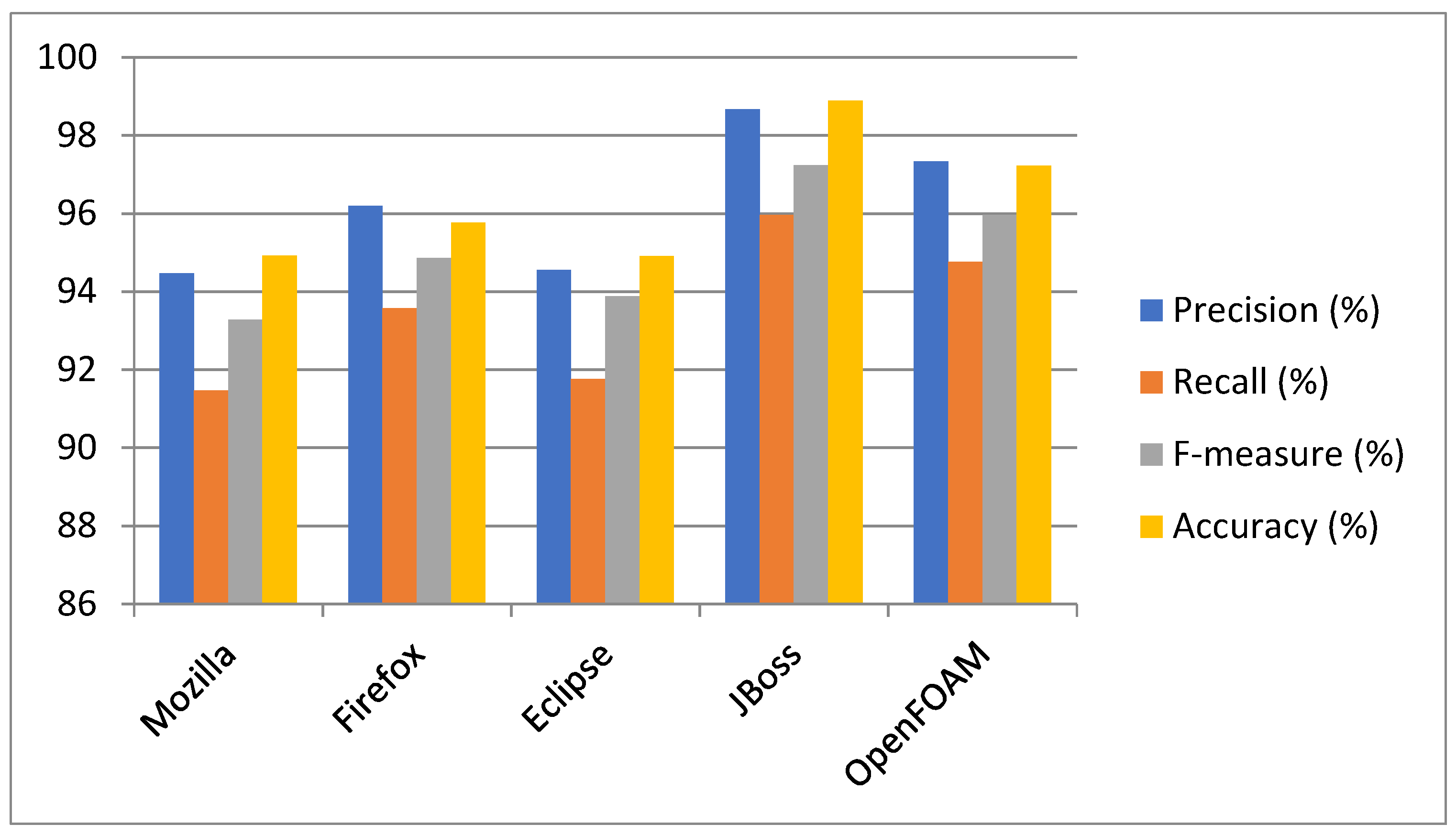
| Projects | Precision (%) | Recall (%) | F-Measure (%) | Accuracy (%) | |
| Proposed BCR | Mozilla | 94.47 | 91.46 | 93.27 | 94.92 |
| Eclipse | 96.19 | 93.57 | 94.86 | 95.76 | |
| JBoss | 94.55 | 91.76 | 93.88 | 94.91 | |
| OpenFOAM | 98.67 | 95.96 | 97.23 | 98.89 | |
| Firefox | 97.33 | 94.76 | 95.96 | 97.22 | |
| Layer | Operator | Output Height | Output Width |
|---|---|---|---|
| Input | 1000 × 200 | 1000 | 200 |
| Dropout | Rate = 0.2 | ||
| Convolutional | Stride = 1, padding = 0, depth = 128, filter size = 20; activation = sigmoid for first four layers, Tanh for last three layers | 128 64 32 | 128 64 32 |
| Pooling | Max pooling | ||
| Fully connected layer | Output depth = Random forest |
| Projects | Zhou et al. | Proposed BCR Model | ||||
|---|---|---|---|---|---|---|
| Precision (%) | Recall (%) | F-Measure (%) | Precision (%) | Recall (%) | F-Measure (%) | |
| Mozilla | 82.60 | 82.40 | 81.70 | 98.48 | 98.52 | 98.12 |
| Eclipse | 81.80 | 82.10 | 81.60 | 99.38 | 99.48 | 99.12 |
| JBoss | 93.70 | 93.70 | 93.70 | 98.88 | 98.95 | 98.42 |
| OpenFOAM | 85.30 | 85.30 | 84.70 | 95.25 | 95.35 | 94.55 |
| Firefox | 80.30 | 80.50 | 79.50 | 92.75 | 92.95 | 91.95 |
© 2019 by the authors. Licensee MDPI, Basel, Switzerland. This article is an open access article distributed under the terms and conditions of the Creative Commons Attribution (CC BY) license (http://creativecommons.org/licenses/by/4.0/).
Share and Cite
Kukkar, A.; Mohana, R.; Nayyar, A.; Kim, J.; Kang, B.-G.; Chilamkurti, N. A Novel Deep-Learning-Based Bug Severity Classification Technique Using Convolutional Neural Networks and Random Forest with Boosting. Sensors 2019, 19, 2964. https://doi.org/10.3390/s19132964
Kukkar A, Mohana R, Nayyar A, Kim J, Kang B-G, Chilamkurti N. A Novel Deep-Learning-Based Bug Severity Classification Technique Using Convolutional Neural Networks and Random Forest with Boosting. Sensors. 2019; 19(13):2964. https://doi.org/10.3390/s19132964
Chicago/Turabian StyleKukkar, Ashima, Rajni Mohana, Anand Nayyar, Jeamin Kim, Byeong-Gwon Kang, and Naveen Chilamkurti. 2019. "A Novel Deep-Learning-Based Bug Severity Classification Technique Using Convolutional Neural Networks and Random Forest with Boosting" Sensors 19, no. 13: 2964. https://doi.org/10.3390/s19132964
APA StyleKukkar, A., Mohana, R., Nayyar, A., Kim, J., Kang, B.-G., & Chilamkurti, N. (2019). A Novel Deep-Learning-Based Bug Severity Classification Technique Using Convolutional Neural Networks and Random Forest with Boosting. Sensors, 19(13), 2964. https://doi.org/10.3390/s19132964