Optimized PID Controller Based on Beetle Antennae Search Algorithm for Electro-Hydraulic Position Servo Control System

Abstract
1. Introduction
2. Related Works
3. Electro-Hydraulic Position Servo Control System
3.1. Working Principles of the System
3.2. Model of the Electro-Hydraulic Position Servo Control System
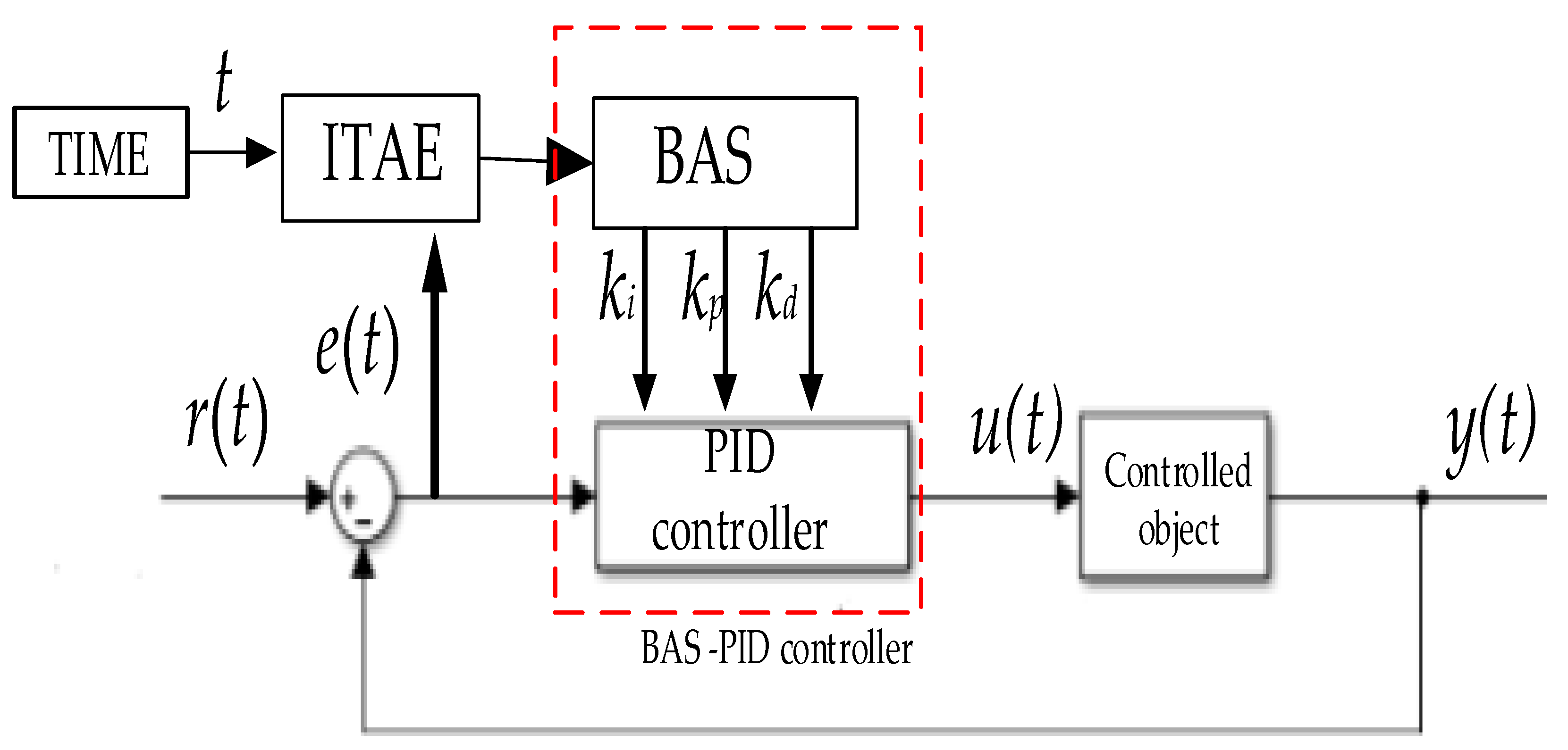
4. BAS-PID Control System
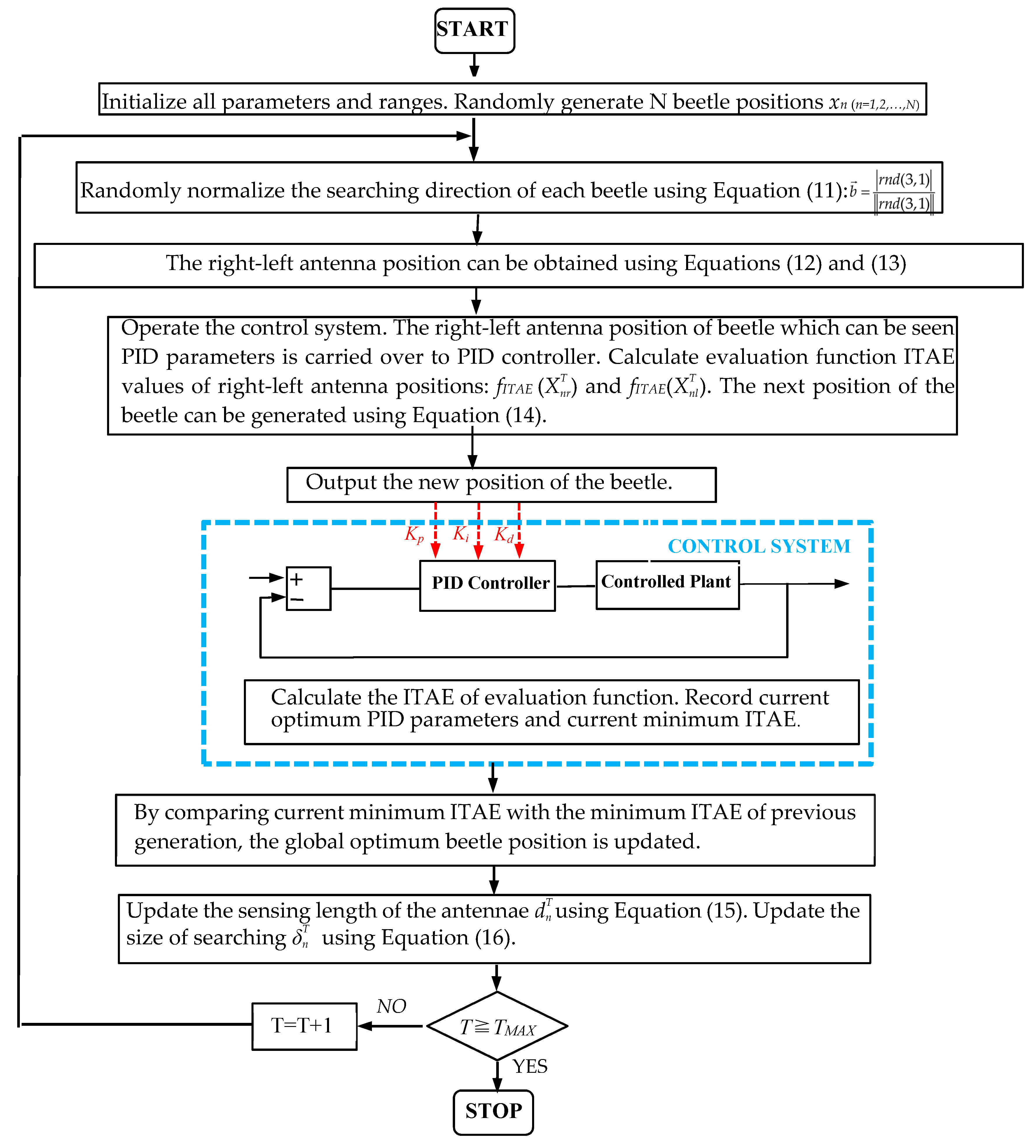
4.1. Beetle Antennae Search Algorithm
| Algorithm 1: BAS |
| Input: Set the maximum number of iterations tmax. Define the evaluation function f(.). Randomly set N beetle positions xti(i = 1, 2, …, N). Set t = 0. Set the value of c according to the optimization purpose. Record the initial sensing length of antennae d0, the initial step size δ0. Record the initial optimum solution, xbest, and the initial optimum value, gbest. |
| Output:xbest, gbest. |
| 1: while (t < Tmax) |
| 2: For i = 1: N |
| 3: Update the searching direction bi using Equation (11) |
| 4: Update the right antenna position xri using Equation (12) |
| 5: Update the left antenna position xli using Equation (13) |
| 6: Update the next position xit+1of the beetle xit using Equation (14). |
| 7: End for |
| 8: For i = 1: N |
| 9: Calculate the function value f(xit+1) of ith beetle. |
| 10: If f(xit+1)is better than gbest |
| 11: xbest = xit+1 |
| 12: gbest = f(xit+1) |
| 13: End if |
| 14: End for |
| 15: Update the sensing length of the antennae dt using Equation (15). |
| 16: Update the step size of searching δt using Equation (16). |
| 17: t = t + 1 |
| 18: End while |
4.2. PID Control System
4.3. System Evaluation Function
4.4. BAS-PID Control System
5. Simulation and Analysis
5.1. Simulation Environment
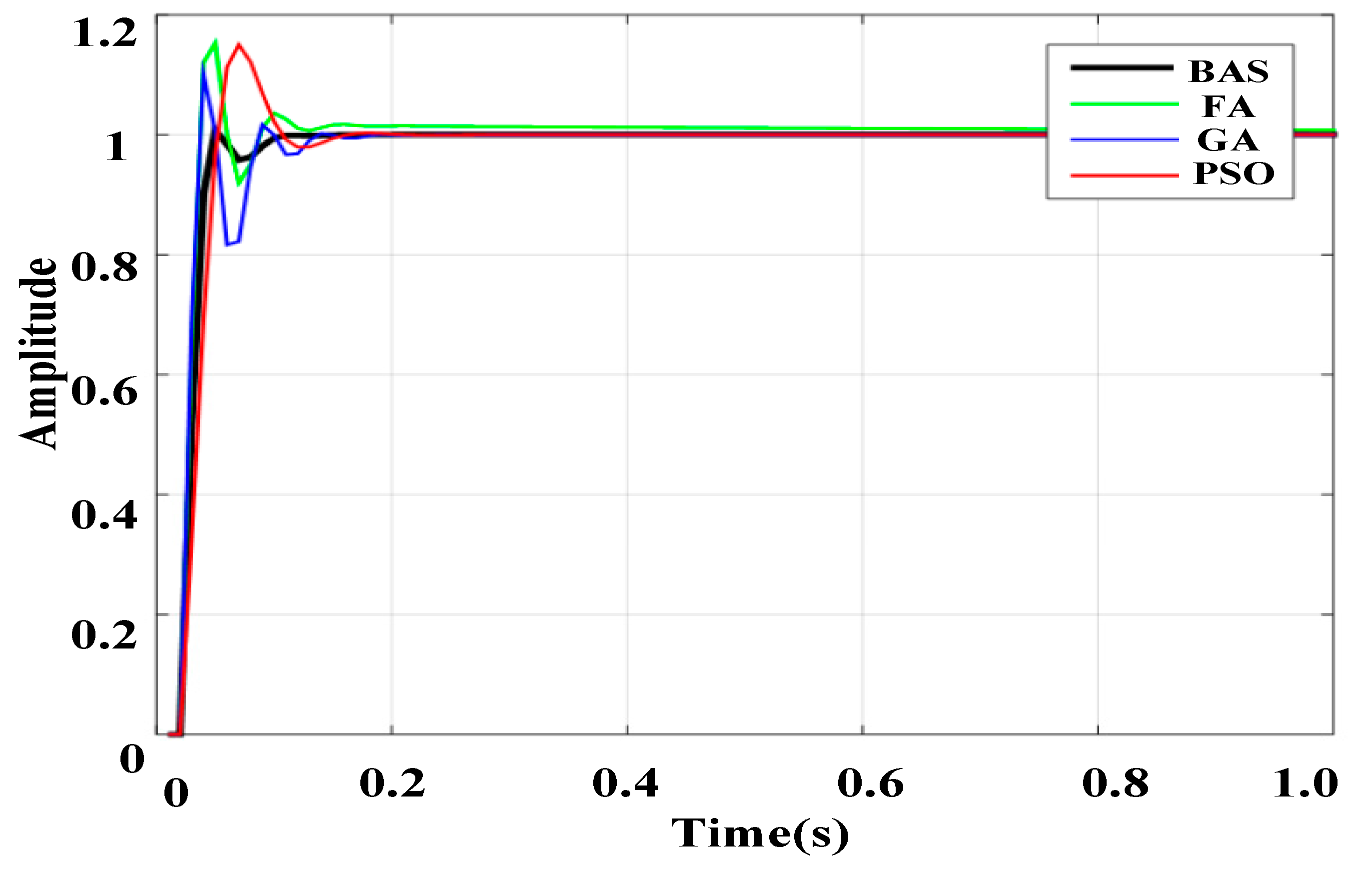
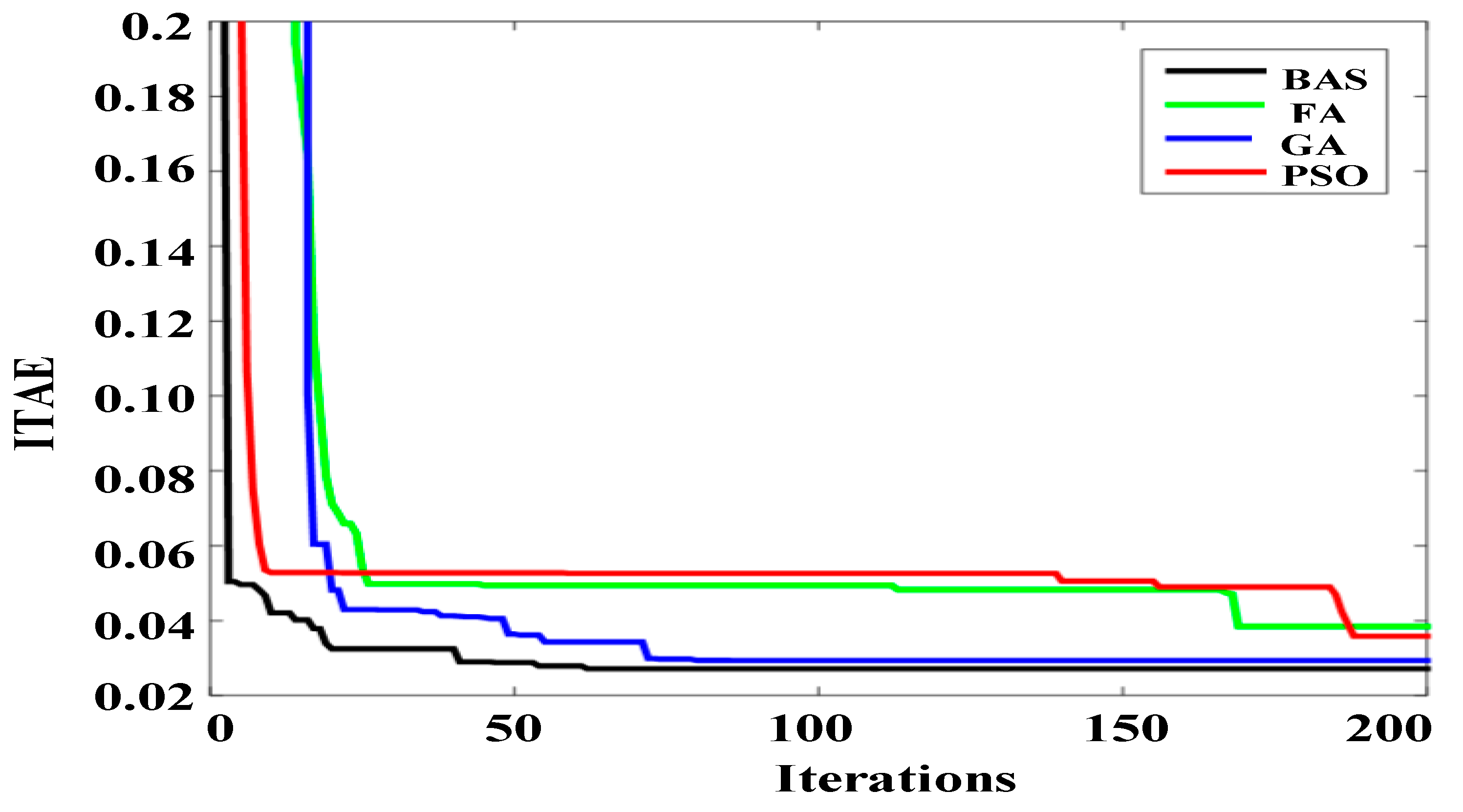
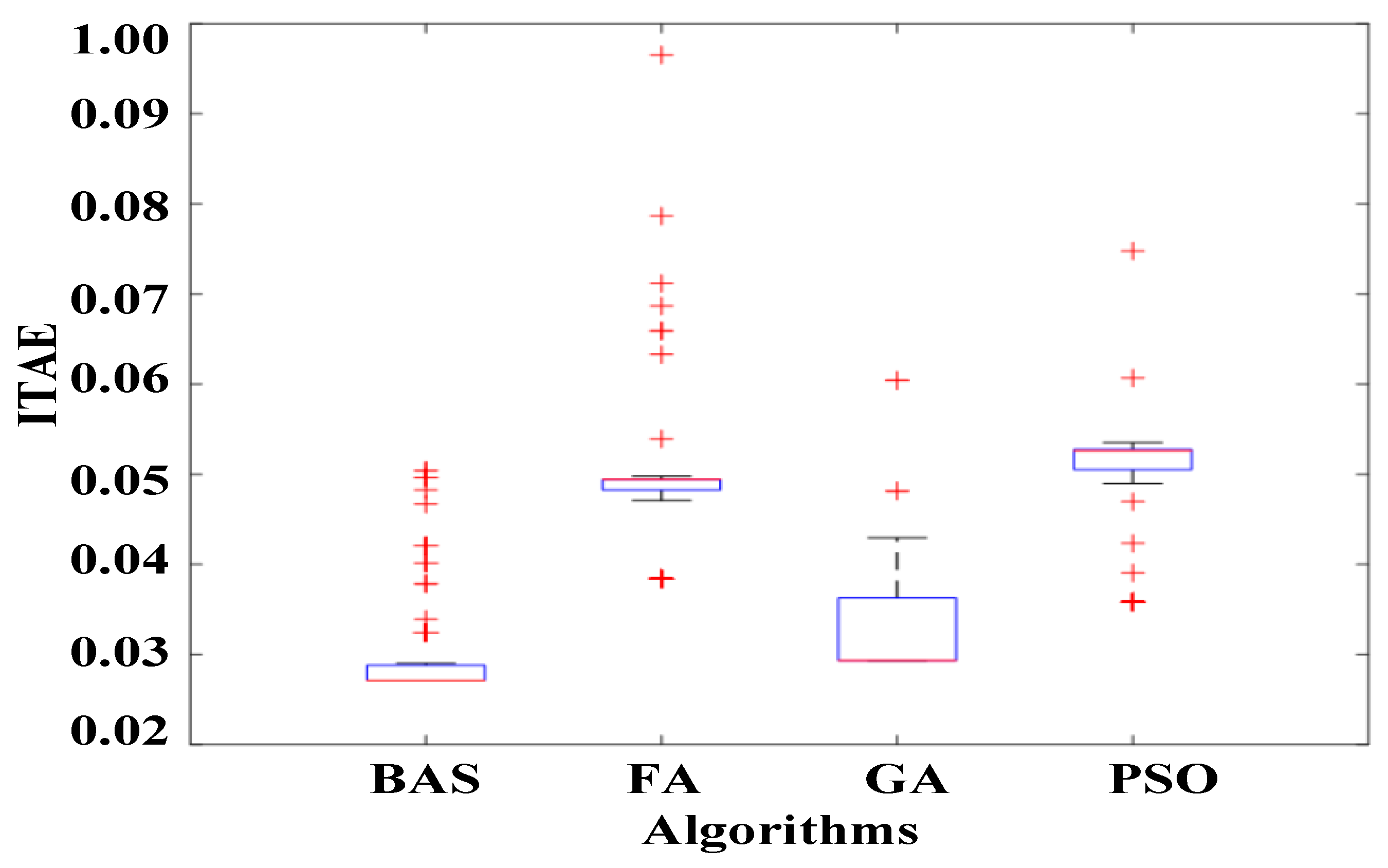
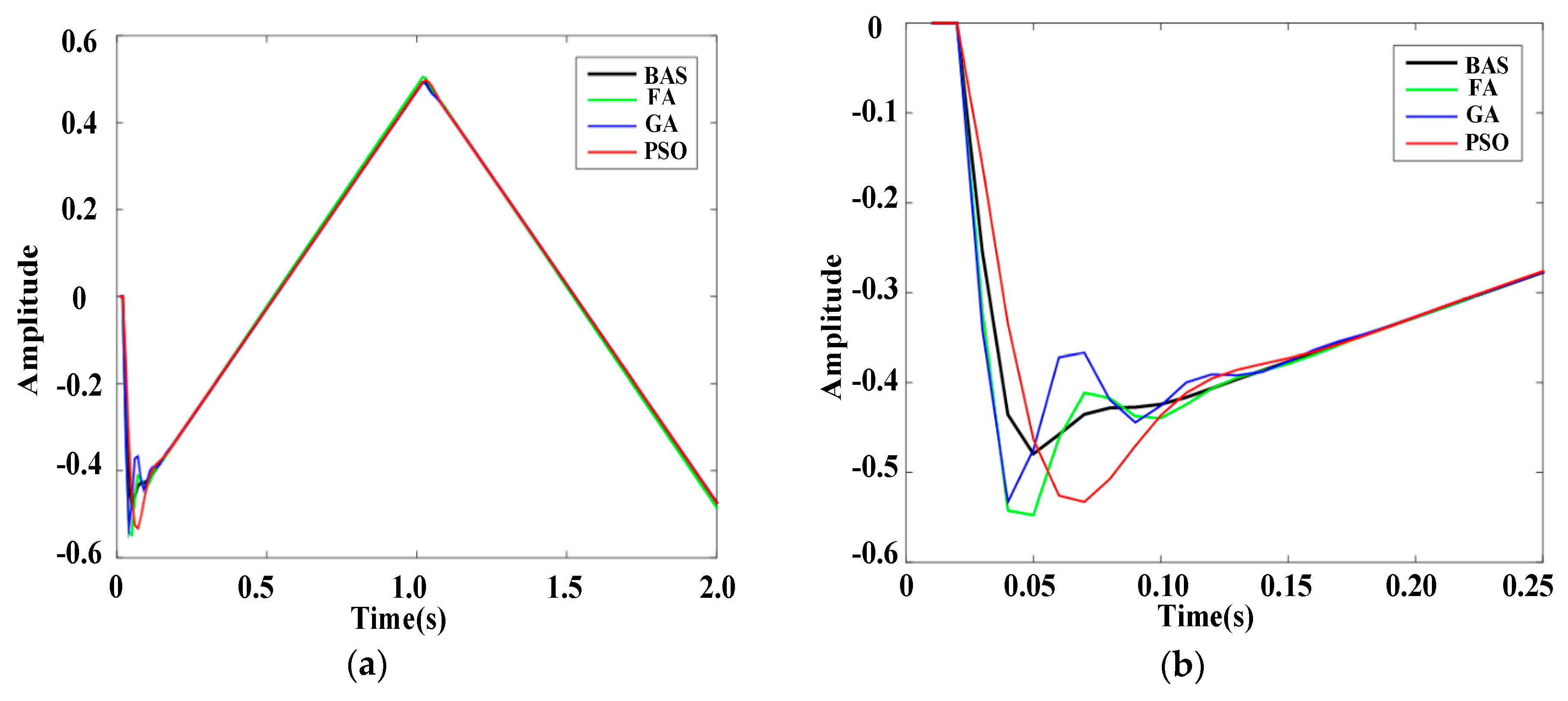
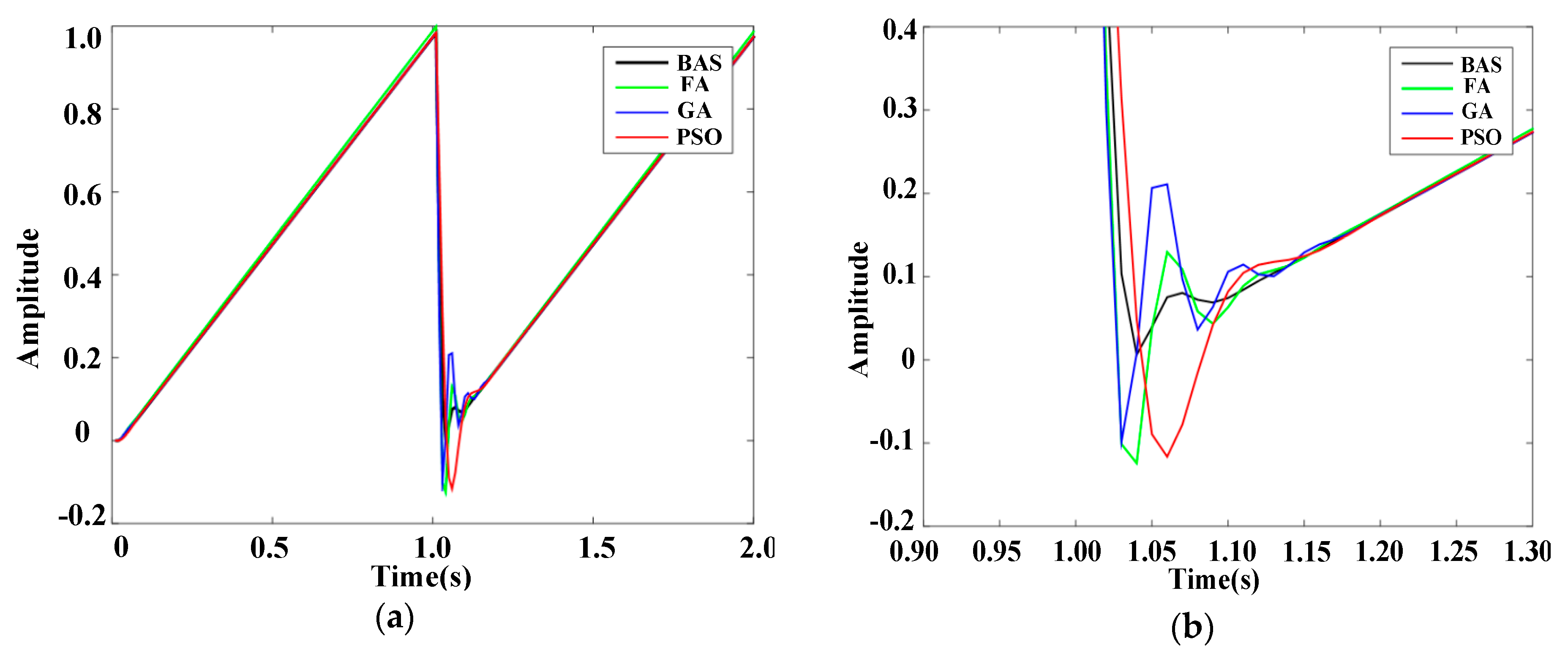
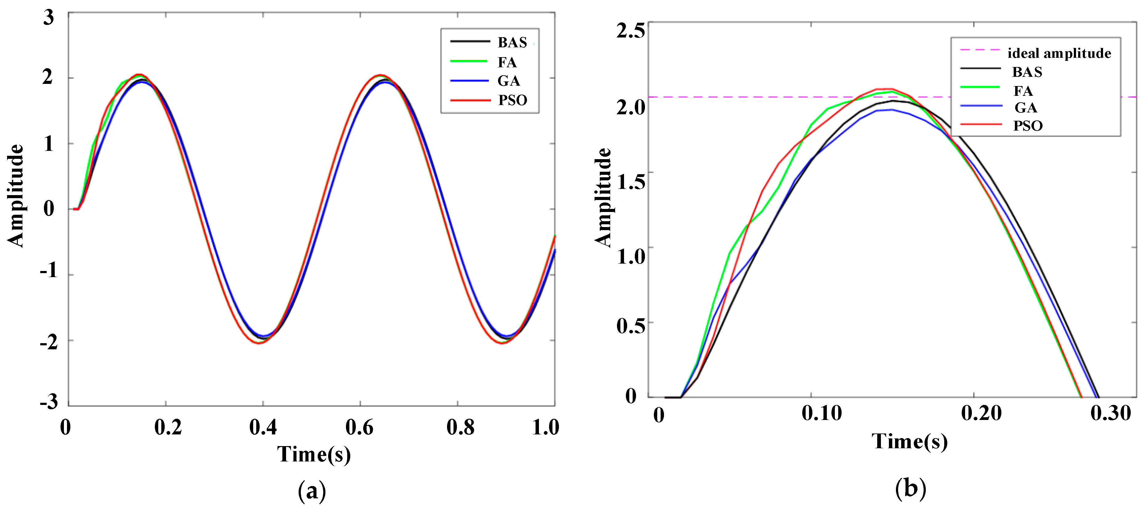
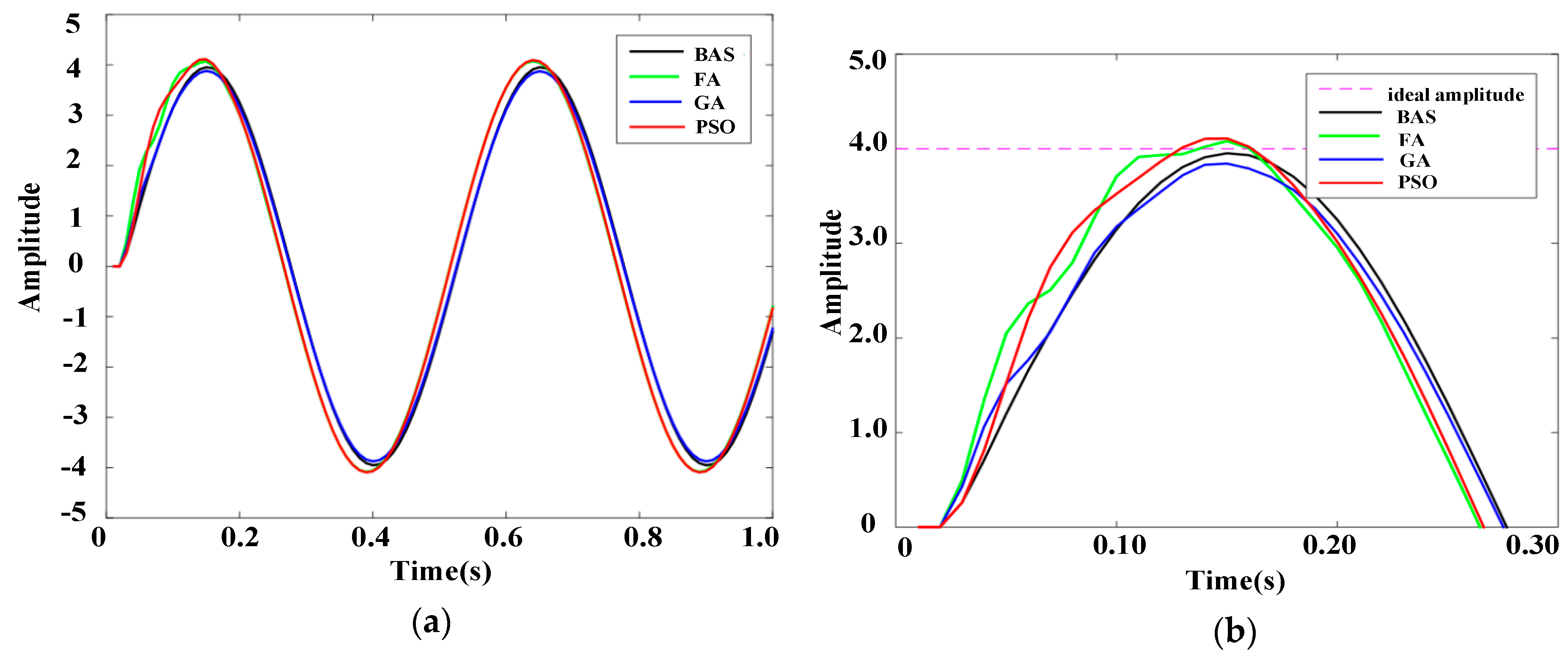
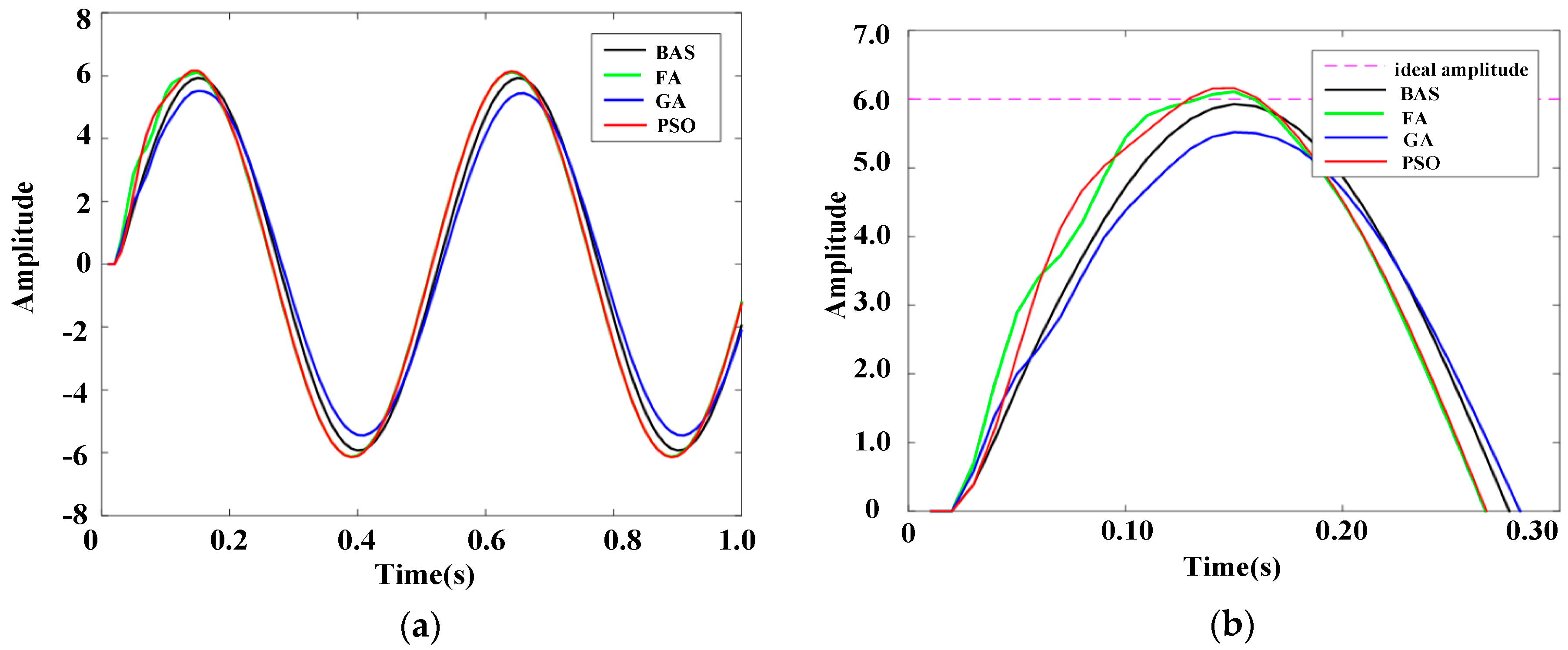
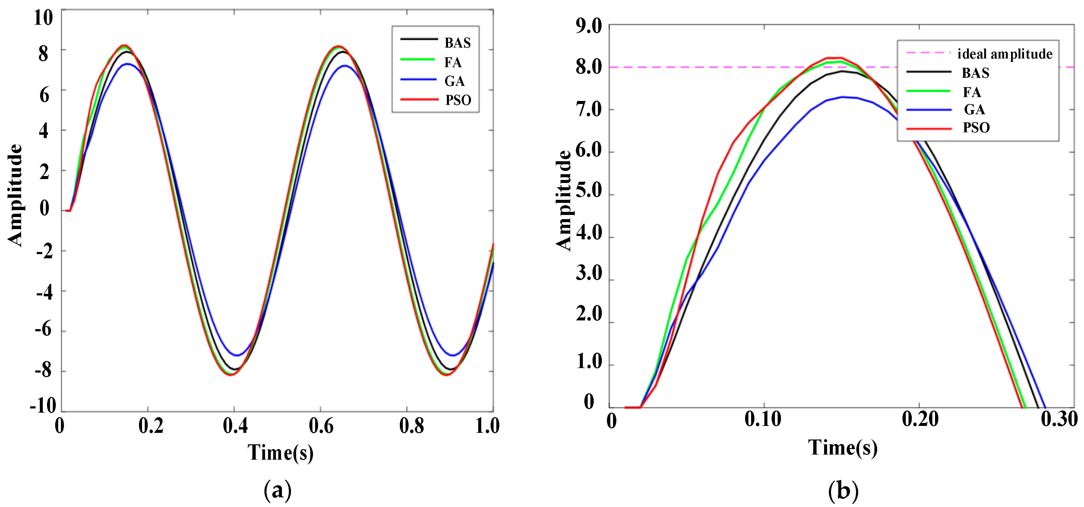
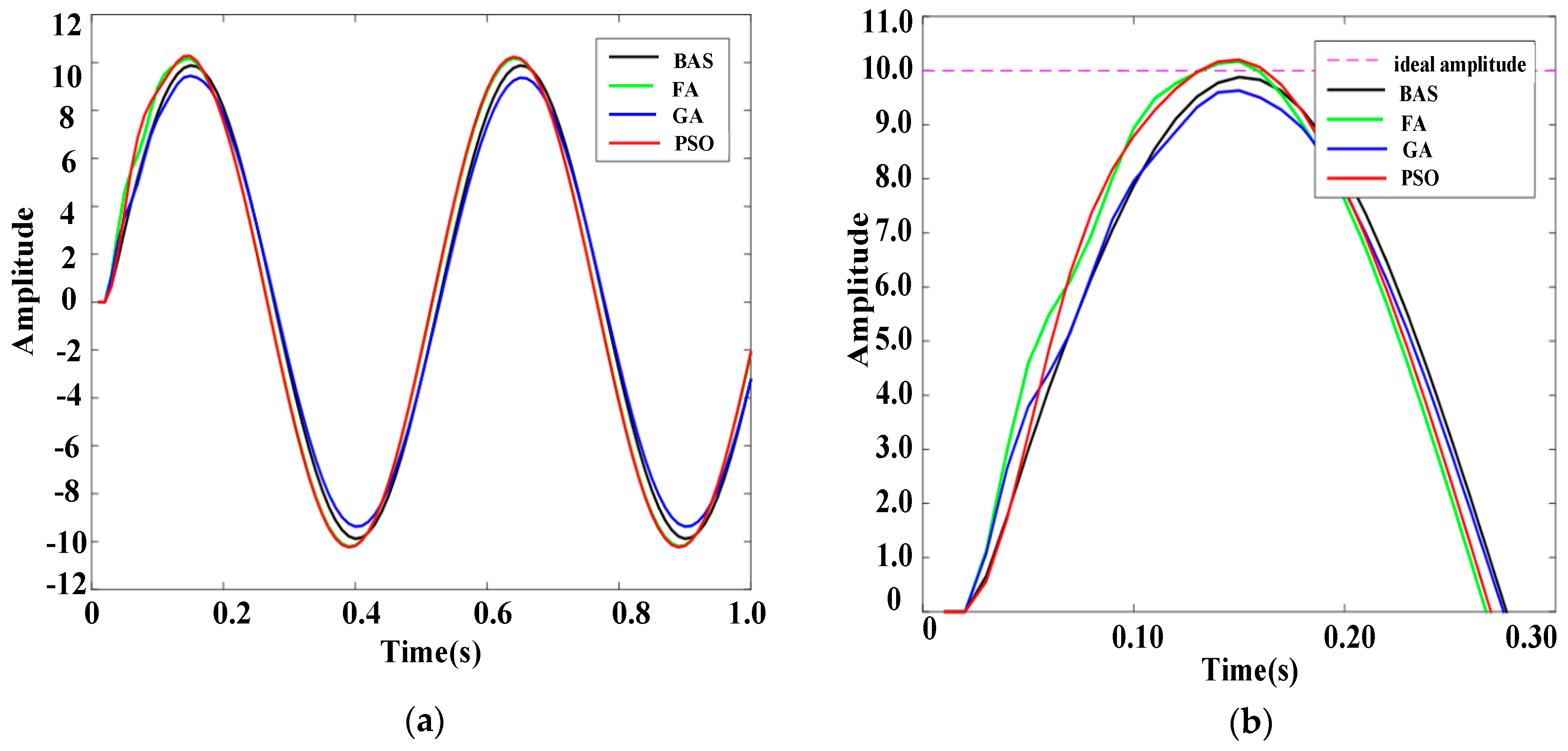
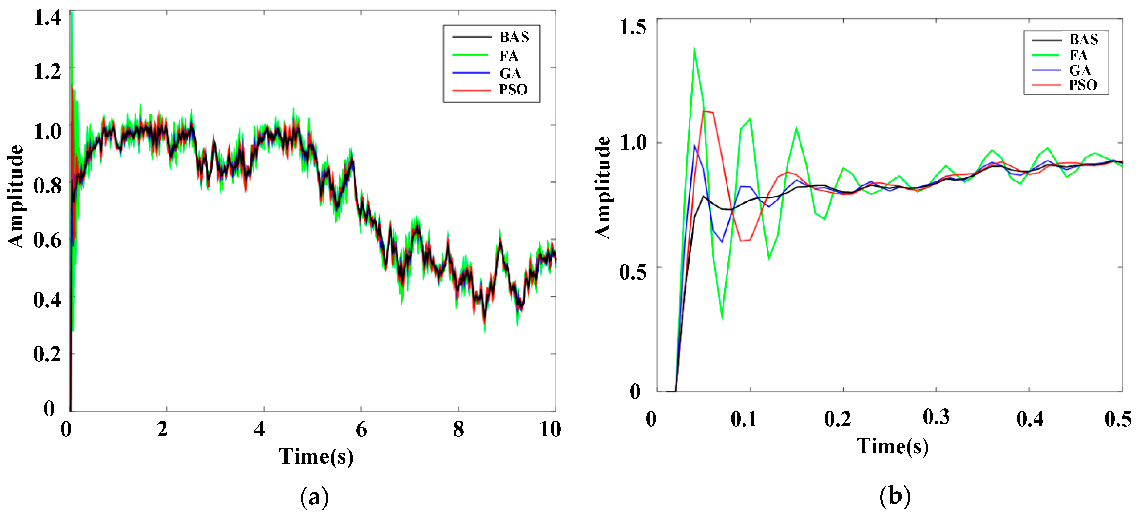
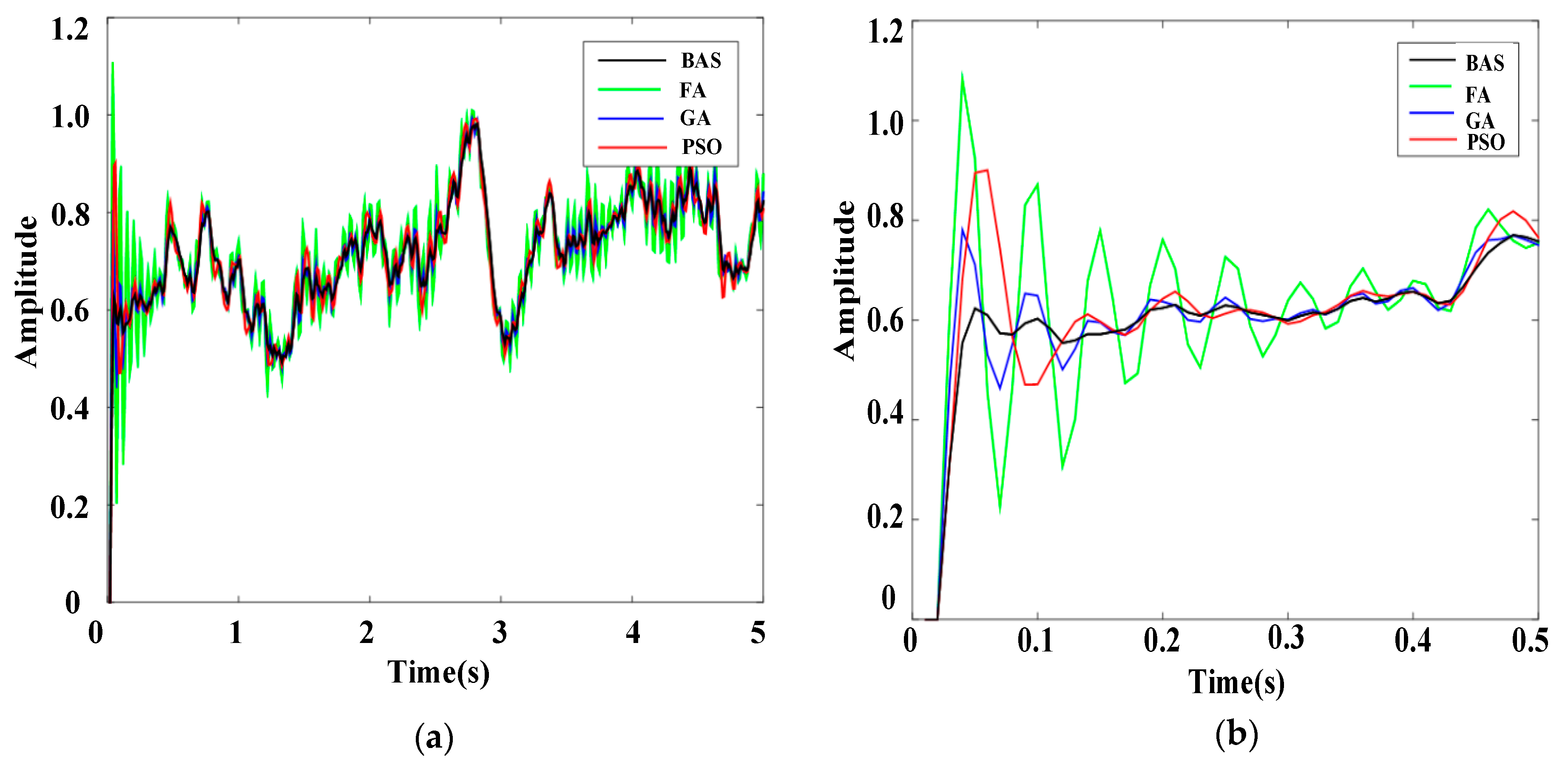
5.2. Simulation Results and Analysis
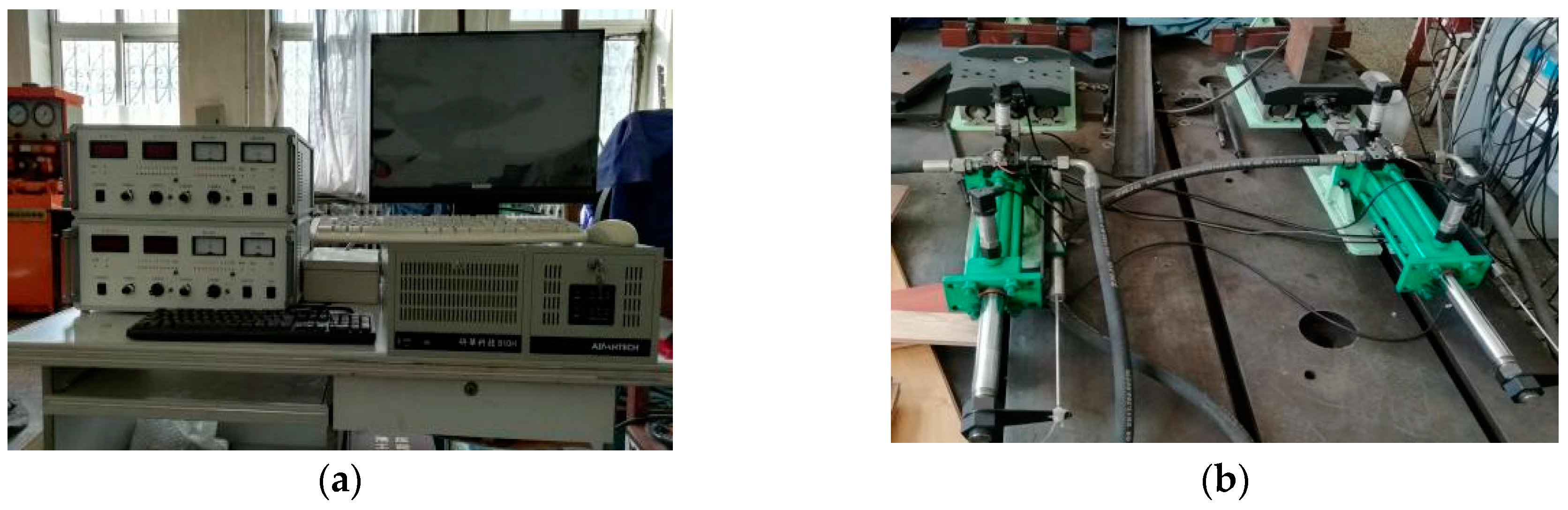
6. Experimental Analysis
7. Conclusions
Author Contributions
Funding
Conflicts of Interest
References
- Yao, J.; Jiao, Z.; Ma, D.; Yan, L. High-Accuracy Tracking Control of Hydraulic Rotary Actuators with Modeling Uncertainties. IEEE ASME Trans. Mechatron. 2014, 19, 633–641. [Google Scholar] [CrossRef]
- Has, Z.; Rahmat, M.F.A.; Husain, A.R.; Ishaque, K.; Ghazali, R.; Ahmad, M.N.; Sam, Y.M.; Rozali, S.M. Robust Position Tracking Control of an Electro-Hydraulic Actuator in the Presence of Friction and Internal Leakage. Arab. J. Sci. Eng. 2013, 39, 2965–2978. [Google Scholar] [CrossRef]
- Yang, G.; Yao, J.; Le, G.; Ma, D. Adaptive integral robust control of hydraulic systems with asymptotic tracking. Mechatronics 2016, 40, 78–86. [Google Scholar] [CrossRef]
- Yuan, H.B.; Na, H.C.; Kim, Y.-B. Robust MPC–PIC force control for an electro-hydraulic servo system with pure compressive elastic load. Control Eng. Pract. 2018, 79, 170–184. [Google Scholar] [CrossRef]
- Wang, D.; Zhao, D.; Gong, M.; Yang, B. Research on Robust Model Predictive Control for Electro-Hydraulic Servo Active Suspension Systems. IEEE Access 2018, 6, 3231–3240. [Google Scholar] [CrossRef]
- Gao, B.; Shao, J.; Yang, X. A compound control strategy combining velocity compensation with ADRC of electro-hydraulic position servo control system. ISA Trans. 2014, 53, 1910–1918. [Google Scholar] [CrossRef] [PubMed]
- Zhao, J.; Wang, Z.; Zhang, C.; Yang, C.; Bai, W.; Zhao, Z. Modal space three-state feedback control for electro-hydraulic servo plane redundant driving mechanism with eccentric load decoupling. ISA Trans. 2018, 77, 201–221. [Google Scholar] [CrossRef] [PubMed]
- Guo, Q.; Shi, G.; He, C.; Wang, D. Composite adaptive force tracking control for electro-hydraulic system without persistent excitation condition. Proc. Inst. Mech. Eng. Part I J. Syst. Control Eng. 2018, 232, 1230–1244. [Google Scholar] [CrossRef]
- Gong, L.; Xiao, C.; Cao, B.; Zhou, Y. Adaptive Smart Control Method for Electric Vehicle Wireless Charging System. Energies 2018, 11, 2685. [Google Scholar] [CrossRef]
- Chen, Q.; Tan, Y.; Li, J.; Mareels, I. Decentralized PID Control Design for Magnetic Levitation Systems Using Extremum Seeking. IEEE Access 2018, 6, 3059–3067. [Google Scholar] [CrossRef]
- Das, J.; Mishra, S.K.; Saha, R.; Mookherjee, S.; Sanyal, D. Nonlinear modeling and PID control through experimental characterization for an electrohydraulic actuation system: System characterization with validation. J. Braz. Soc. Mech. Sci. Eng. 2016, 39, 1177–1187. [Google Scholar] [CrossRef]
- Ghosh, B.B.; Sarkar, B.K.; Saha, R. Realtime performance analysis of different combinations of fuzzy–PID and bias controllers for a two degree of freedom electrohydraulic parallel manipulator. Robot. Comput.-Integr. Manuf. 2015, 34, 62–69. [Google Scholar] [CrossRef]
- Zhang, Y.; Zhang, L.; Dong, Z. An MEA-Tuning Method for Design of the PID Controller. Math. Probl. Eng. 2019, 2019, 1378783. [Google Scholar] [CrossRef]
- Yang, X.; Chen, X.; Xia, R.; Qian, Z. Wireless Sensor Network Congestion Control Based on Standard Particle Swarm Optimization and Single Neuron PID. Sensors 2018, 18, 1265. [Google Scholar] [CrossRef] [PubMed]
- Fister, D.; Fister, I.; Fister, I.; Šafarič, R. Parameter tuning of PID controller with reactive nature-inspired algorithms. Robot. Auton. Syst. 2016, 84, 64–75. [Google Scholar] [CrossRef]
- Wang, X.; Yan, X.; Li, D.; Sun, L. An Approach for Setting Parameters for Two-Degree-of-Freedom PID Controllers. Algorithms 2018, 11, 48. [Google Scholar] [CrossRef]
- Ziegler, J.; Nichols, N. Optimum settings for automatic controllers. J. Dyn. Syst. Meas. Control 1993, 115, 220–222. [Google Scholar] [CrossRef]
- Hajare, V.D.; Patre, B.M.; Khandekar, A.A.; Malwatkar, G.M. Decentralized PID controller design for TITO processes with experimental validation. Int. J. Dyn. Control 2016, 5, 583–595. [Google Scholar] [CrossRef]
- Elbayomy, K.M.; Zongxia, J.; Huaqing, Z. PID Controller Optimization by GA and Its Performances on the Electro-hydraulic Servo Control System. Chin. J. Aeronaut. 2008, 21, 378–384. [Google Scholar] [CrossRef]
- Cheng, C.-H.; Cheng, P.-J.; Xie, M.-J. Current sharing of paralleled DC–DC converters using GA-based PID controllers. Expert Syst. Appl. 2010, 37, 733–740. [Google Scholar] [CrossRef]
- Ye, Y.; Yin, C.-B.; Gong, Y.; Zhou, J.-J. Position control of nonlinear hydraulic system using an improved PSO based PID controller. Mech. Syst. Signal Proc. 2017, 83, 241–259. [Google Scholar] [CrossRef]
- Wang, R.; Tan, C.; Xu, J.; Wang, Z.; Jin, J.; Man, Y. Pressure Control for a Hydraulic Cylinder Based on a Self-Tuning PID Controller Optimized by a Hybrid Optimization Algorithm. Algorithms 2017, 10, 19. [Google Scholar] [CrossRef]
- Rajesh, K.S.; Dash, S.S.; Rajagopal, R. Hybrid improved firefly-pattern search optimized fuzzy aided PID controller for automatic generation control of power systems with multi-type generations. Swarm Evol. Comput. 2019, 44, 200–211. [Google Scholar] [CrossRef]
- Pradhan, P.C.; Sahu, R.K.; Panda, S. Firefly algorithm optimized fuzzy PID controller for AGC of multi-area multi-source power systems with UPFC and SMES. Int. J. Eng. Sci. Technol. 2016, 19, 338–354. [Google Scholar] [CrossRef]
- Gheisarnejad, M. An effective hybrid harmony search and cuckoo optimization algorithm based fuzzy PID controller for load frequency control. Appl. Soft Comput. 2018, 65, 121–138. [Google Scholar] [CrossRef]
- Sahoo, B.P.; Panda, S. Improved grey wolf optimization technique for fuzzy aided PID controller design for power system frequency control. Energy Grids Netw. 2018, 16, 278–299. [Google Scholar] [CrossRef]
- Ünal, M.; Erdal, H.; Topuz, V. Trajectory tracking performance comparison between genetic algorithm and ant colony optimization for PID controller tuning on pressure process. Comput. Appl. Eng. Educ. 2012, 20, 518–528. [Google Scholar] [CrossRef]
- Goher, K.M.; Fadlallah, S.O. Bacterial foraging-optimized PID control of a two-wheeled machine with a two-directional handling mechanism. Robot. Biomim. 2017, 4, 1. [Google Scholar] [CrossRef]
- Jiang, X.; Li, S. BAS: Beetle Antennae Search Algorithm for Optimization Problems. Int. J. Robot. Control 2018, 1, 1–5. [Google Scholar] [CrossRef]
- Sun, Y.; Zhang, J.; Li, G.; Wang, Y.; Sun, J.; Jiang, C. Optimized neural network using beetle antennae search for predicting the unconfined compressive strength of jet grouting coalcretes. Int. J. Numer. Anal. Methods Geomech. 2019, 43, 801–813. [Google Scholar] [CrossRef]
- Zhu, Z.; Zhang, Z.; Man, W.; Tong, X.; Qiu, J.; Li, F. A new beetle antennae search algorithm for multi-objective energy management in microgrid. In Proceedings of the 13th IEEE Conference on Industrial Electronics and Applications, Wuhan, China, 31 May–2 June 2018. [Google Scholar]
- Chen, T.; Zhu, Y.; Teng, J. Beetle swarm optimisation for solving investment portfolio problems. J. Eng. 2018, 16, 1600–1605. [Google Scholar] [CrossRef]
- Fei, S.-W.; He, C.-X. Prediction of dissolved gases content in power transformer oil using BASA-based mixed kernel RVR model. Int. J. Green Energy 2019, 16, 652–656. [Google Scholar] [CrossRef]
- Sun, Y.; Zhang, J.; Li, G.; Ma, G.; Huang, Y.; Sun, J.; Wang, Y.; Nener, B. Determination of Young’s modulus of jet grouted coalcretes using an intelligent model. Eng. Geol. 2019, 252, 43–53. [Google Scholar] [CrossRef]
- Sun, J.; Zhang, J.; Gu, Y.; Huang, Y.; Sun, Y.; Ma, G. Prediction of permeability and unconfined compressive strength of pervious concrete using evolved support vector regression. Constr. Build. Mater. 2019, 207, 440–449. [Google Scholar] [CrossRef]
- Jiang, X.; Li, S. Beetle Antennae Search without Parameter Tuning (BAS-WPT) for Multi-objective Optimization. arXiv 2017, arXiv:1711.02395v1. [Google Scholar]
- Wu, Q.; Shen, X.; Jin, Y.; Chen, Z.; Li, S.; Khan, A.H.; Chen, D. Intelligent Beetle Antennae Search for UAV Sensing and Avoidance of Obstacles. Sensors 2019, 19, 2112. [Google Scholar] [CrossRef]
- Lin, M.; Li, Q. A Hybrid Optimization Method of Beetle Antennae Search Algorithm and Particle Swarm Optimization. In Proceedings of the 2018 International Conference on Electrical, Control, Automation and Robotics, Xiamen, China, 16–17 September 2018. [Google Scholar]
- Li, Q.; Wei, A.; Zhang, Z. Application of Economic Load Distribution of Power System Based on BAS-PSO. In Proceedings of the 2nd International Symposium on Application of Materials Science and Energy Materials, Shanghai, China, 17–18 December 2018. [Google Scholar]
- Liu, Q.; Wang, Z.; Wei, A. Research on Optimal Scheduling of Wind-PV-Hydro-Storage Power Complementary System Based on BAS Algorithm. In Proceedings of the 2nd International Symposium on Application of Materials Science and Energy Materials, Shanghai, China, 17–18 December 2018. [Google Scholar]
- Wang, C.; Ren, C.; Li, B.; Wang, Y.; Wang, K. Research on Straightness Error Evaluation Method Based on Search Algorithm of Beetle. In Proceedings of the 8th International Workshop of Advanced Manufacturing and Automation, Changzhou, China, 25–26 September 2018. [Google Scholar]
- Zhang, Y.; Li, S.; Xu, B. Convergence analysis of beetle antennae search algorithm and its applications. arXiv 2019, arXiv:1904.02397. [Google Scholar]
- Bartoszewicz, A.; Nowacka-Leverton, A. ITAE Optimal Sliding Modes for Third-Order Systems with Input Signal and State Constraints. IEEE Trans. Autom. Control 2010, 55, 1928–1932. [Google Scholar] [CrossRef]
- Xu, J.X.; Chen, L.; Chang, C.H. Tuning of fuzzy PI controllers based on gain/phase margin specifications and ITAE index. ISA Trans. 1996, 35, 79–91. [Google Scholar]
- Nowackaleverton, A.; Bartoszewicz, A. ITAE optimal variable structure control of second order systems with input signal and velocity constraints. Kybernetes 2009, 38, 1093–1105. [Google Scholar] [CrossRef]
- Guha, D.; Roy, P.K.; Banerjee, S. Load frequency control of interconnected power system using grey wolf optimization. Swarm Evol. Comput. 2016, 27, 97–115. [Google Scholar] [CrossRef]
- Rajasekhar, A.; Jatoth, R.K.; Abraham, A. Design of intelligent PID/PIλDμ speed controller for chopper fed DC motor drive using opposition based artificial bee colony algorithm. Eng. Appl. Artif. Intell. 2014, 29, 13–32. [Google Scholar] [CrossRef]
- Yousefi, H.; Handroos, H.; Soleymani, A. Application of Differential Evolution in system identification of a servo-hydraulic system with a flexible load. Mechatronics 2008, 18, 513–528. [Google Scholar] [CrossRef]
- Ba, K.; Yu, B.; Gao, Z.; Li, W.; Ma, G.; Kong, X. Parameters Sensitivity Analysis of Position-Based Impedance Control for Bionic Legged Robots’ HDU. Appl. Sci. 2017, 7, 1035. [Google Scholar] [CrossRef]
- Kong, X.; Yu, B.; Quan, L.; Ba, K.; Wu, L. Nonlinear mathematical modeling and sensitivity analysis of hydraulic drive unit. Chin. J. Mech. Eng. 2015, 28, 999–1011. [Google Scholar] [CrossRef]
- Xu, Z.; Gao, J.; Li, H.; Liu, H.; Li, X.; Liu, Y.; Sun, W.; Zhao, W. The modeling and controlling of electrohydraulic actuator for quadruped robot based on fuzzy Proportion Integration Differentiation controller. Proc. Inst. Mech. Eng. Part C J. Eng. Mech. Eng. Sci. 2014, 228, 2557–2568. [Google Scholar] [CrossRef]


| BAS Variants | Variant Way | Advantages |
|---|---|---|
| BPNN-BAS [30] | • BAS was used to train back propagation neural network (BPNN) | • High BPNN training speed • Make weights optimal |
| PSO-BAS [32,38,39] | • BAS was combined with PSO | • Greater global search ability • Better searching capacity than that of standard PSO |
| BAS-MkRVR [33] | • BAS was used to select the appropriate kernel parameters and controlled parameters of the mixed kernel relevance vector regression (MkRVR) | • Stronger prediction capacity than RBFRVR and Sigmoid RVR. |
| SVM-BAS [34] | • The hyper-parameters of the support vector machine (SVM) were firstly tuned by BAS | • Less time-consuming • Low-cost • Non-destructive |
| ESVR-BAS [35] | • The hyper-parameters of the evolved support vector regression was tuned by BAS | • More efficient than random hyper-parameter selection • High predictive capability |
| BAS-WPT [36] | • Normalization method and penalty function method were used to extend BAS | • Not require prior parameter tuning • Simple to design, implement, and has less complexity |
| OABAS [37] | • OABAS was designed on the basic of BAS to improve the path planning | • Wider search range and the breakneck search speed • Shorter path length |
| Contrastive Algorithms | Advantages of BAS | Relevant Recent References |
|---|---|---|
| PSO | Faster iteration speed Stronger ability to jump local optimal solution | [32,37,38,39] |
| GA | Does not need binary to represent decimal numbers The BAS program runs faster | [39] |
| FA | Does not need more initial parameters BAS program code simple | This paper |
| BA | Simple to implement, and has less complexity | [42] |
| ABC | Higher efficiency Lower time complexity | [37] |
| BAS | FA | GA | PSO | |
|---|---|---|---|---|
| Kp | 7.9927 | 9.5773 | 8.0156 | 8.2923 |
| Ki | 0.1412 | 6.9449 | 0 | 0.0225 |
| Kd | 0.0532 | 0.0714 | 0.0978 | 0 |
| ITAE | 0.0275 | 0.0384 | 0.0294 | 0.0358 |
| Mp | 0.0067 | 0.1439 | 0.1015 | 0.1503 |
| tr | 0.022 | 0.051 | 0.056 | 0.029 |
| td | 0.023 | 0.026 | 0.029 | 0.036 |
| Amplitude | Index | BAS | PSO | GA | FA |
|---|---|---|---|---|---|
| 2 | Aω | 0.9870 | 1.0270 | 0.9695 | 1.0165 |
| ∆Aω | 0.0130 | 0.0270 | 0.0305 | 0.0165 | |
| 4 | Aω | 0.9878 | 1.0267 | 0.9693 | 1.0175 |
| ∆Aω | 0.0122 | 0.0267 | 0.0307 | 0.0175 | |
| 6 | Aω | 0.9878 | 1.0271 | 0.9186 | 1.0177 |
| ∆Aω | 0.0122 | 0.0271 | 0.0814 | 0.0177 | |
| 8 | Aω | 0.9879 | 1.0267 | 0.9878 | 1.0174 |
| ∆Aω | 0.0121 | 0.0267 | 0.0122 | 0.0174 | |
| 10 | Aω | 0.9878 | 1.0191 | 0.9696 | 1.0190 |
| ∆Aω | 0.0122 | 0.0191 | 0.0304 | 0.0190 |
© 2019 by the authors. Licensee MDPI, Basel, Switzerland. This article is an open access article distributed under the terms and conditions of the Creative Commons Attribution (CC BY) license (http://creativecommons.org/licenses/by/4.0/).
Share and Cite
Fan, Y.; Shao, J.; Sun, G. Optimized PID Controller Based on Beetle Antennae Search Algorithm for Electro-Hydraulic Position Servo Control System. Sensors 2019, 19, 2727. https://doi.org/10.3390/s19122727
Fan Y, Shao J, Sun G. Optimized PID Controller Based on Beetle Antennae Search Algorithm for Electro-Hydraulic Position Servo Control System. Sensors. 2019; 19(12):2727. https://doi.org/10.3390/s19122727
Chicago/Turabian StyleFan, Yuqi, Junpeng Shao, and Guitao Sun. 2019. "Optimized PID Controller Based on Beetle Antennae Search Algorithm for Electro-Hydraulic Position Servo Control System" Sensors 19, no. 12: 2727. https://doi.org/10.3390/s19122727
APA StyleFan, Y., Shao, J., & Sun, G. (2019). Optimized PID Controller Based on Beetle Antennae Search Algorithm for Electro-Hydraulic Position Servo Control System. Sensors, 19(12), 2727. https://doi.org/10.3390/s19122727