Optimizing Charging Efficiency and Maintaining Sensor Network Perpetually in Mobile Directional Charging


Abstract
:1. Introduction
- As far as we know, this is the first work investigating the mobile directional charging problem in WRSN aiming to maximize the energy charging efficiency and maintain the networks working continuously.
- We prove that the problem is NP-hard.
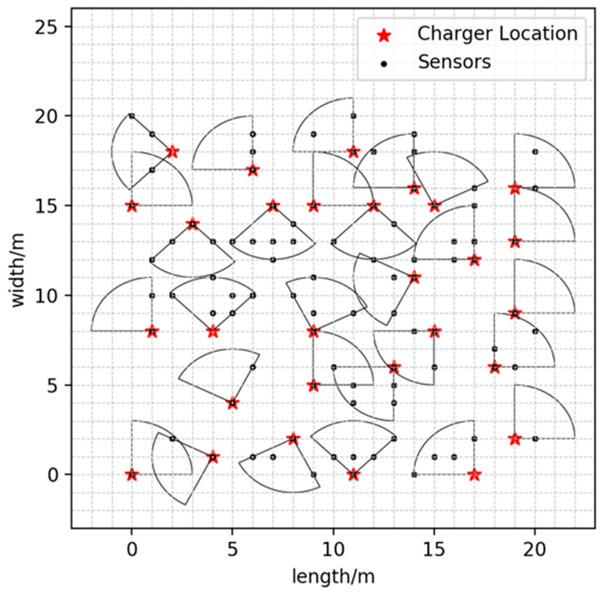
- We propose the coverage utility of the DCV’s directional charging, and design an approximation algorithm to determine the docking spots and their charging orientations while minimizing the number of the DCV’s docking spots and maximizing the charging coverage utility. It ensures the mobile charging coverage for all the sensors in the network and improves the energy charging efficiency locally.
- We propose a moving path planning algorithm for the DCV’s mobile charging to optimize the DCV’s energy charging efficiency while ensuring the networks working continuously.
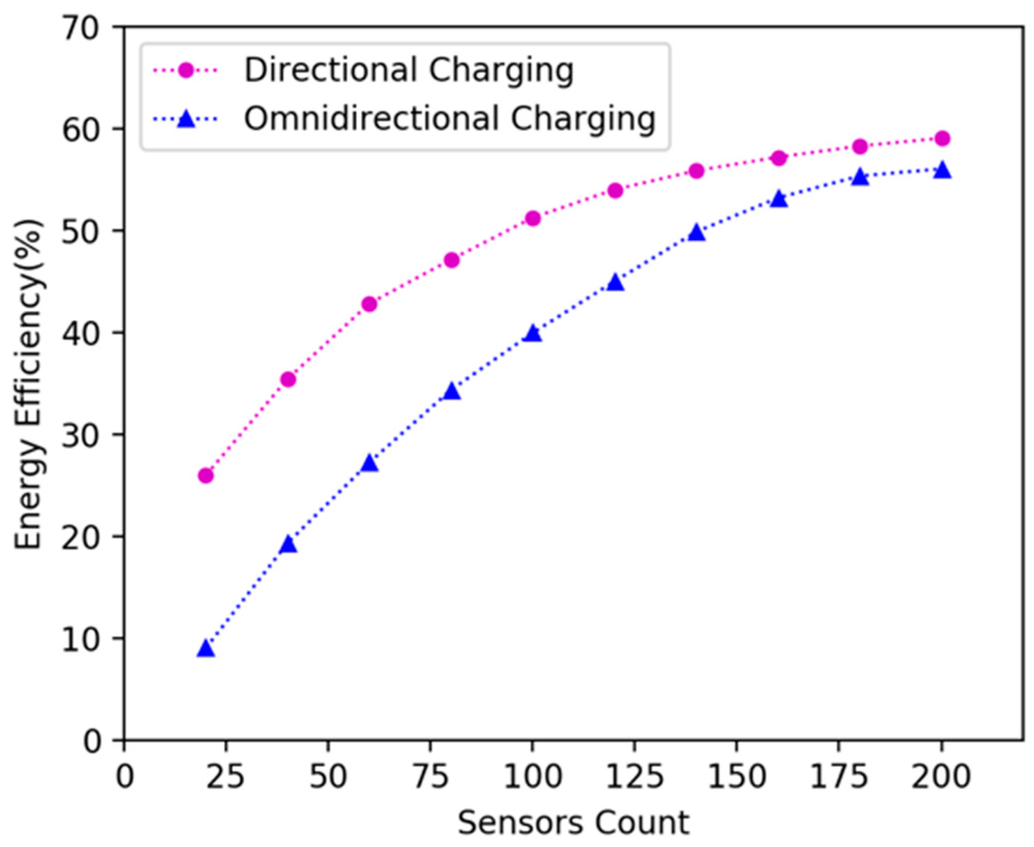
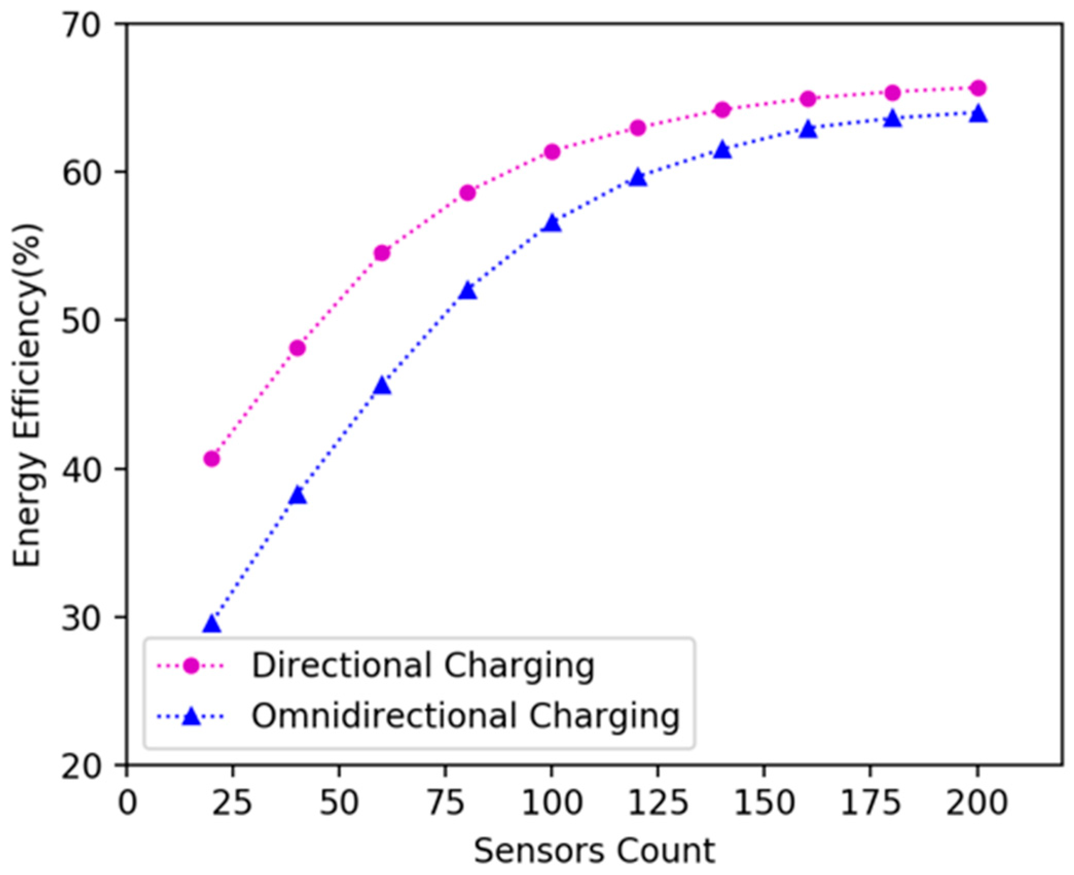
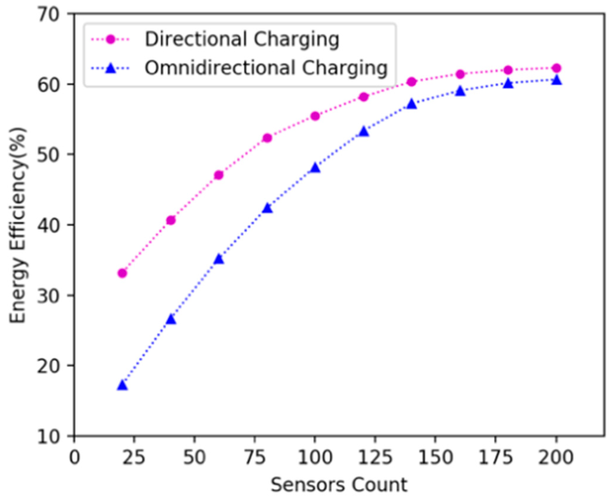
- We theoretically analyze the DCV’s charging service capability, and perform the comprehensive simulation experiments. The experiment results show that energy charging efficiency is higher than omnidirectional charging model in the data collection network.
2. Related Works
3. Problem Formation
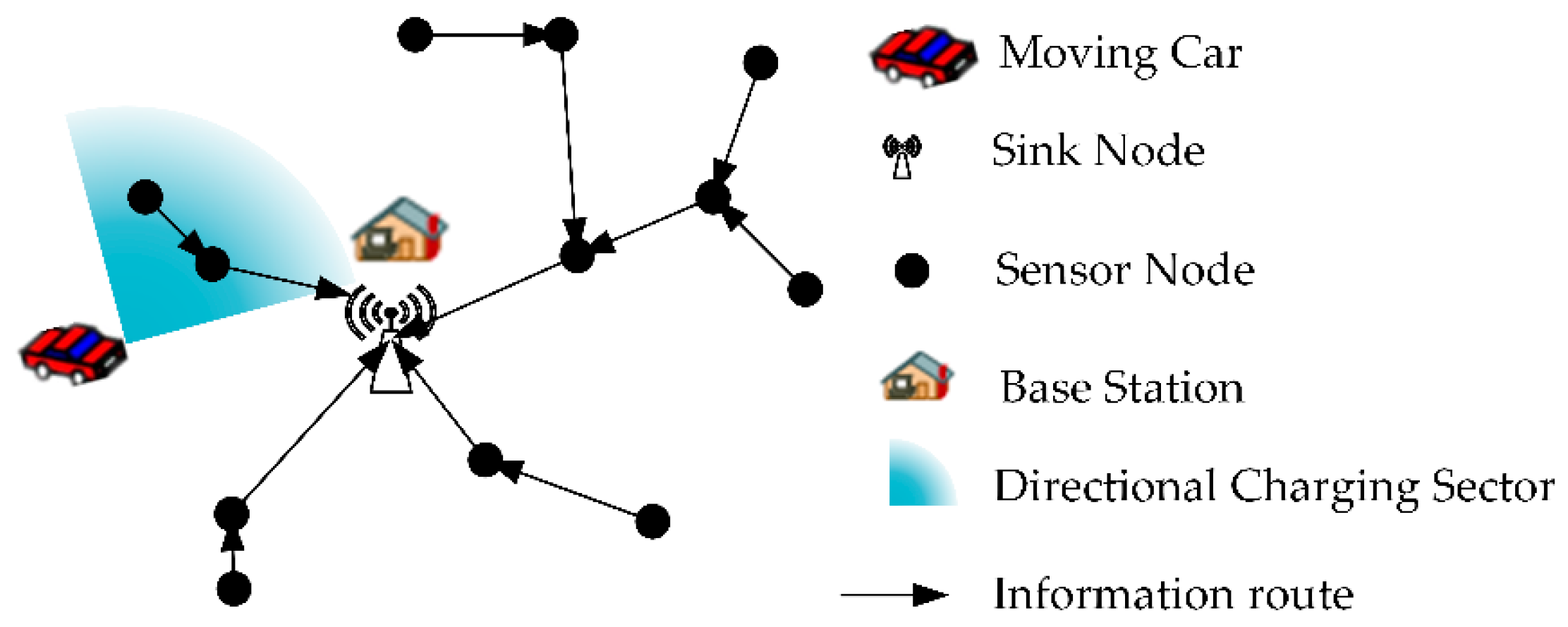
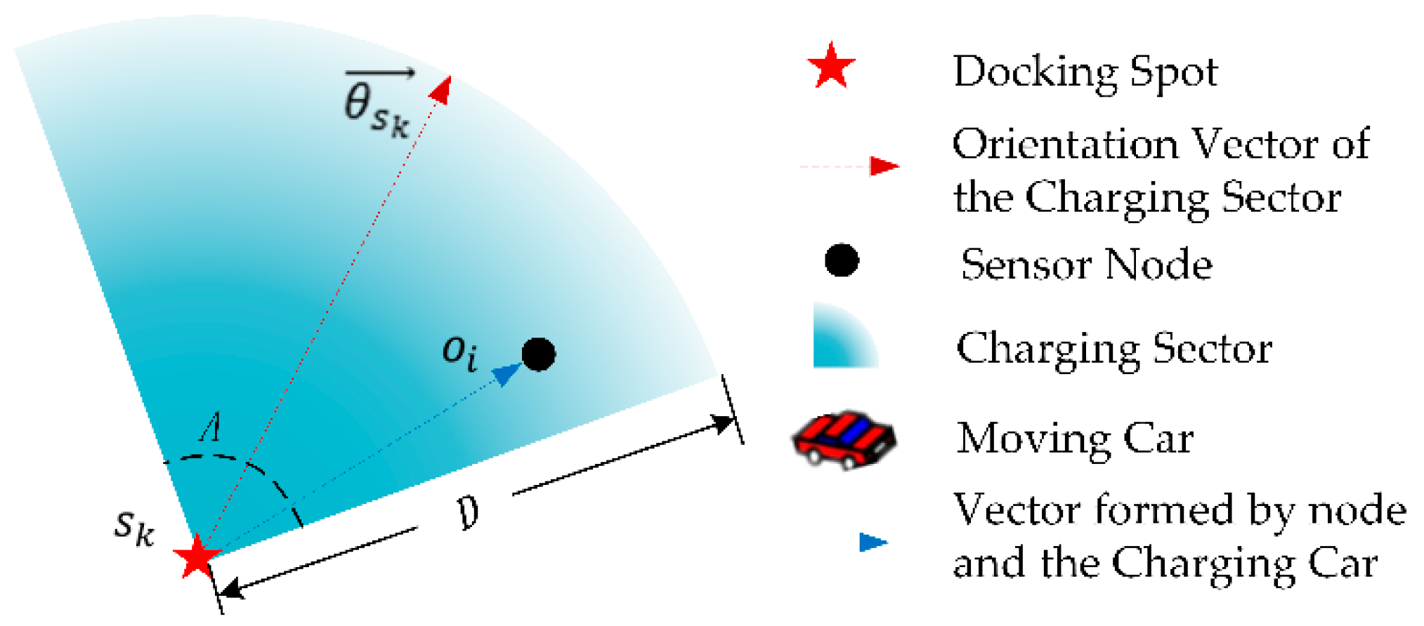
3.1. Directional Charging Model
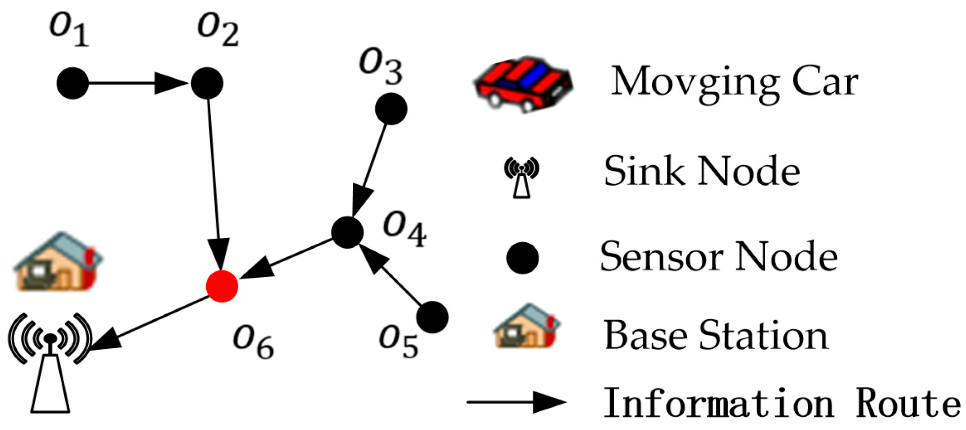
3.2. Network Energy Consumption Model
3.3. Problem Formulation
4. Design and Analysis of Algorithms
- (1)
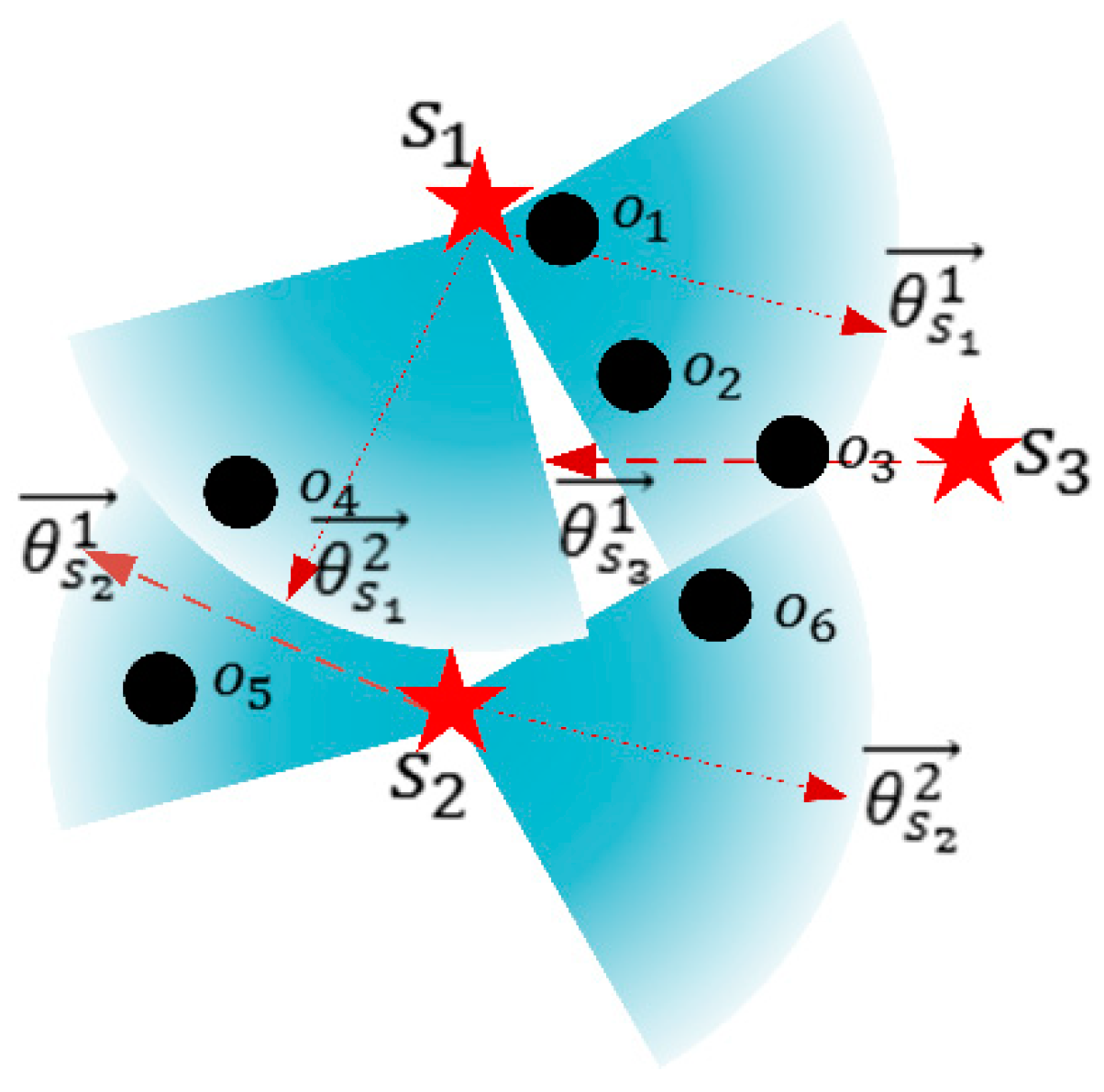
- First, we find the set of Docking Spots () and their corresponding Charging Orientation () to maximize the charging coverage utility and ensure the mobile charging coverage of the network (Section 3.1).
- (2)
- Second, we plan the DCV’s charging path to travel through all docking spot in DS and the charging residence time at each docking spot to optimize the overall energy charging efficiency while maintaining the sensor network working continuously (Section 3.2).
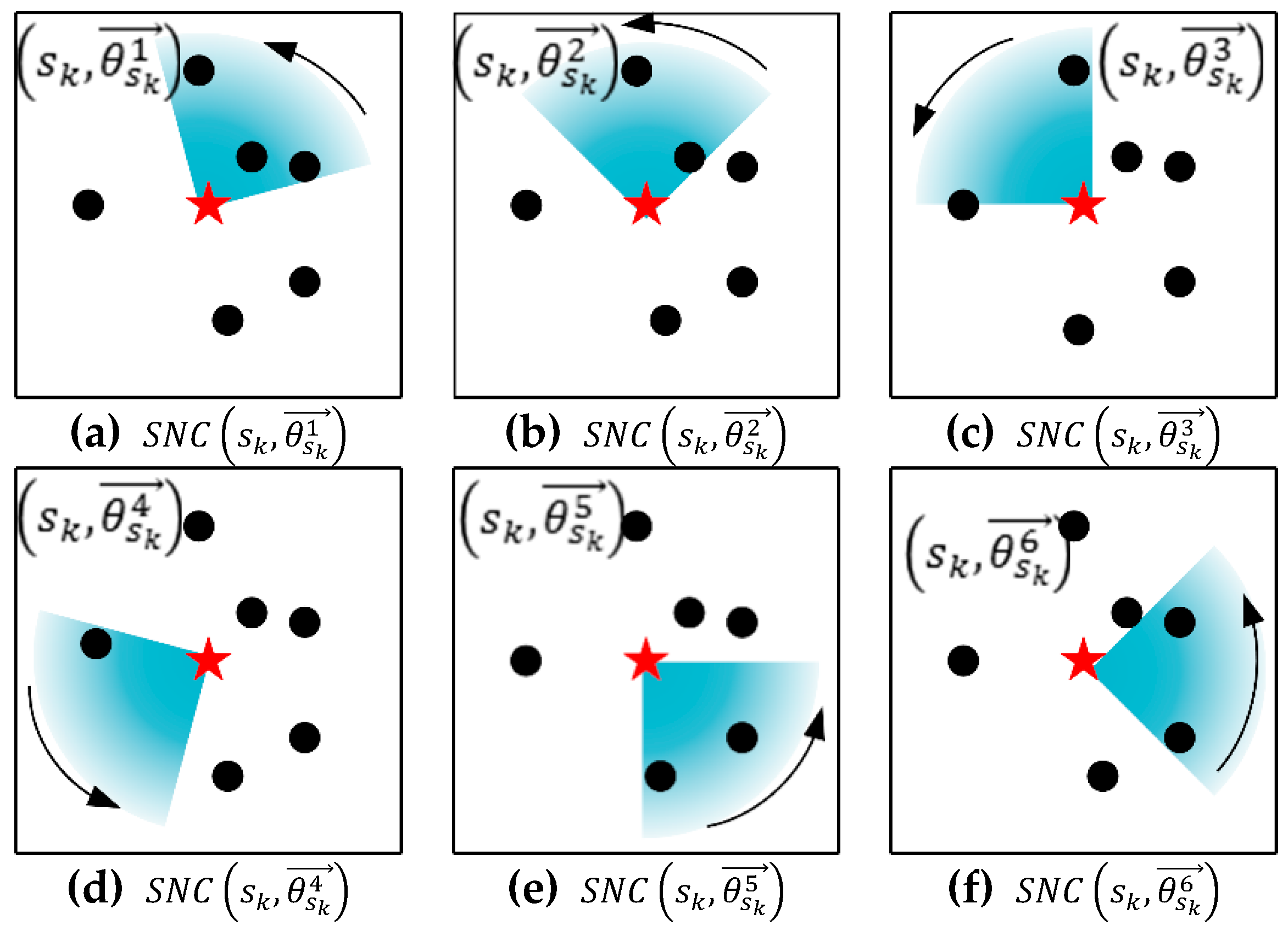
4.1. Find Charging Docking Spots and Charging Directions
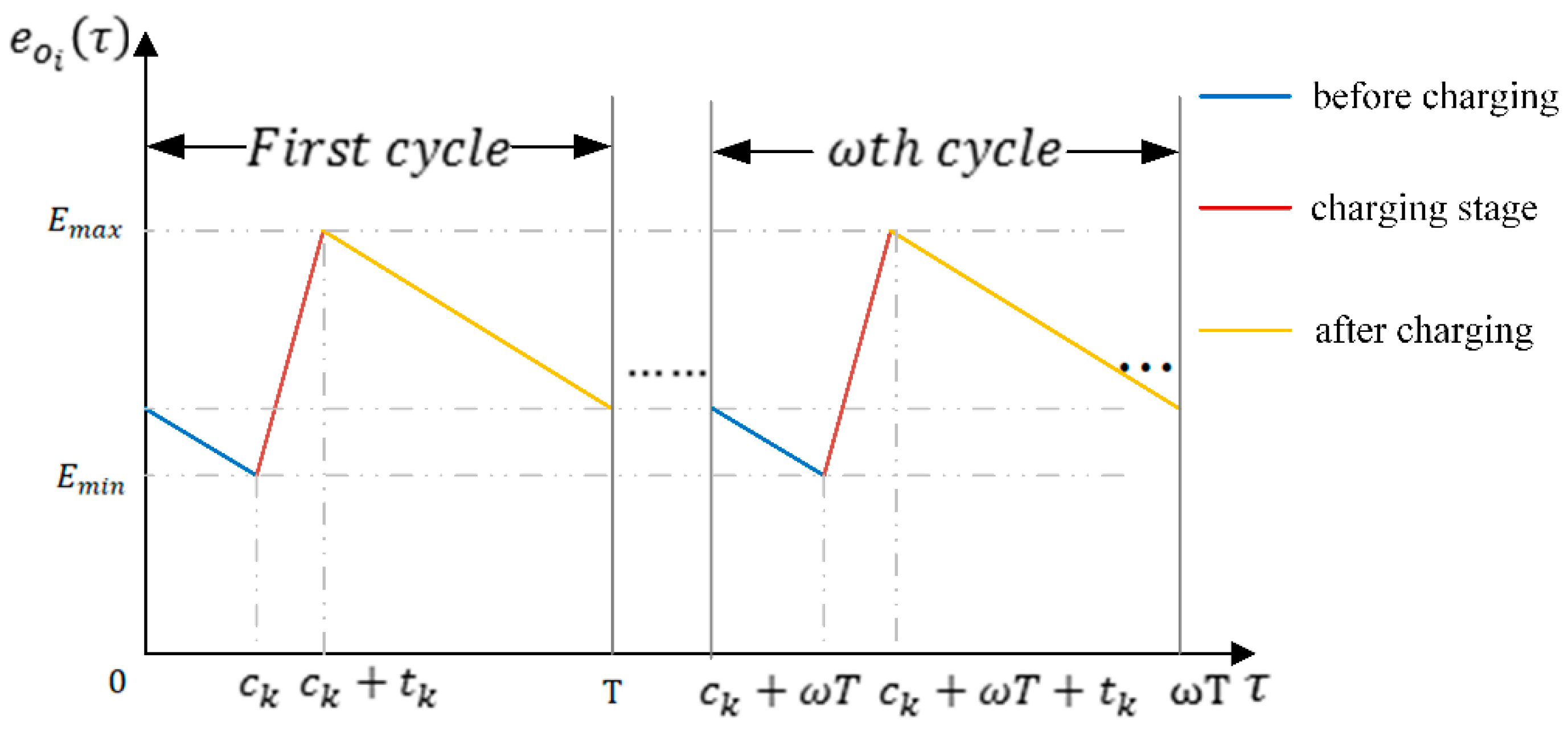
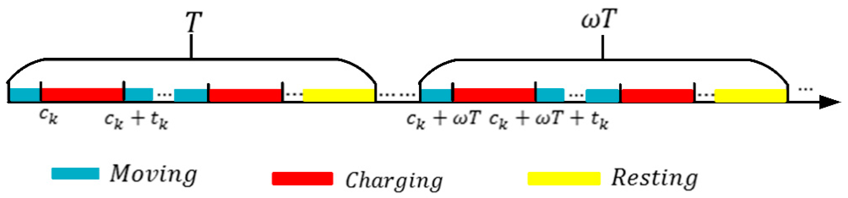
4.2. Plan Moving Path and Charging Residence Time
- (1)
- The energy received by a sensor is greater or equal to the energy consumed in a charging cycle;
- (2)
- The residual energy value of a node will not be lower than during a charging cycle.
5. Analysis of the DCV’s Service Capability
6. Simulation Experiments
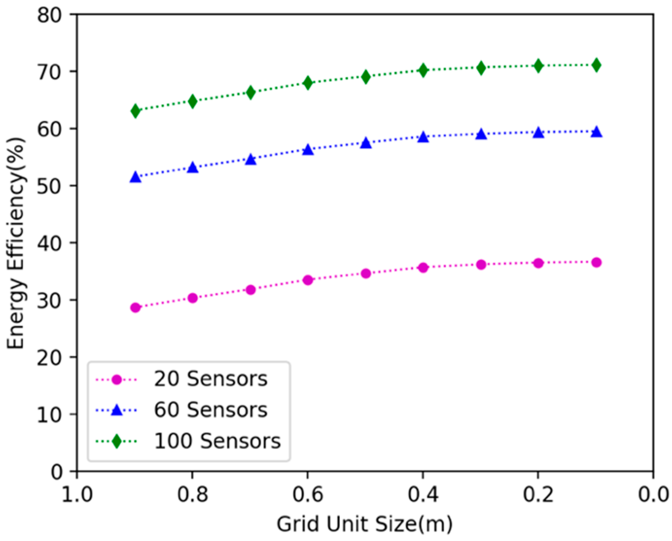
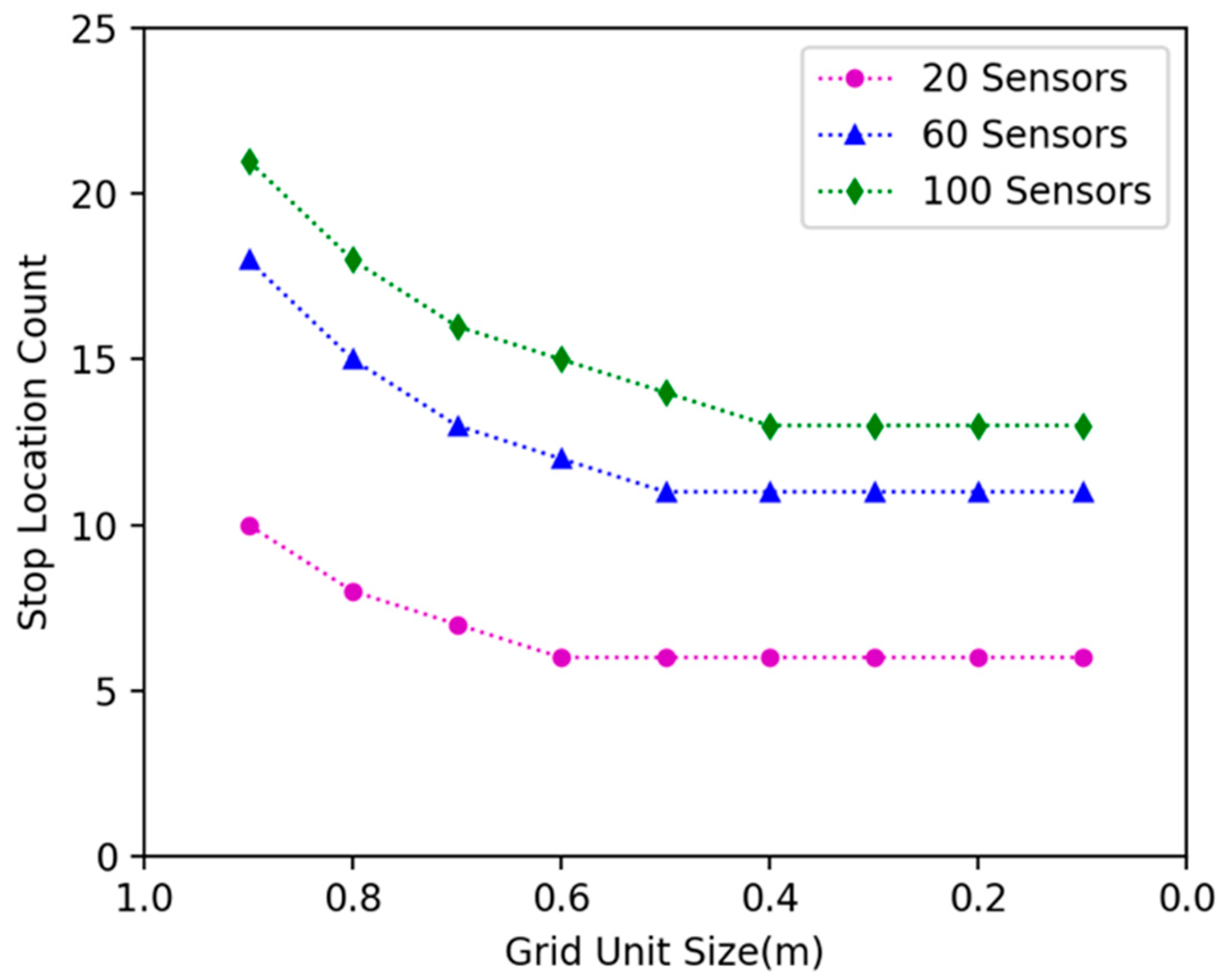
6.1. Comparison Experiments on Different Grid Size
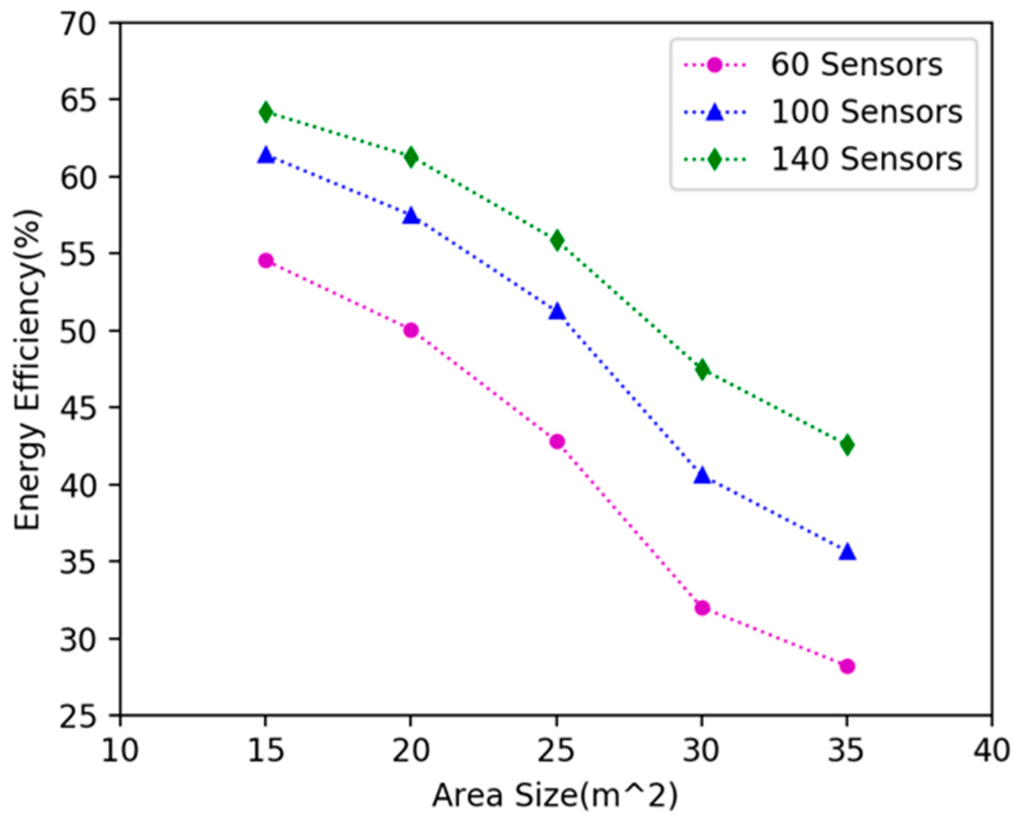
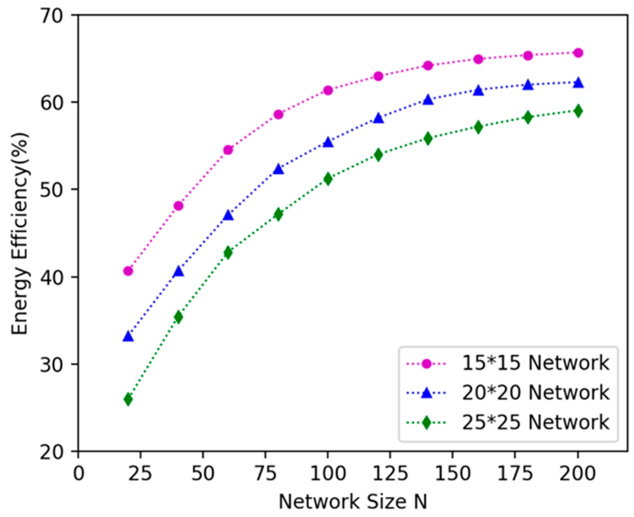
6.2. Comparison Experiments on Different Network Size And Area Size
6.3. Comparison Experiments on Mobile Omnidirectional and Directional Charging
7. Conclusions
Author Contributions
Funding
Conflicts of Interest
References
- Kurs, A.; Moffatt, R.; Soljacic, M. Simultance mid-range power transfer to multiple devices. Appl. Phys. Lett. 2010, 96, 34. [Google Scholar] [CrossRef]
- André, K.; Aristeidis, K.; Robert, M.; Joannopoulos, J.D.; Peter, F.; Marin, S. Wireless power transfer via strongly coupled magnetic resonances. Science 2007, 317, 83–86. [Google Scholar]
- Valenta, C.R.; Durgin, G.D. Harvesting Wireless Power: Survey of Energy-Harvester Conversion Efficiency in Far-Field, Wireless Power Transfer Systems. IEEE Microw. Mag. 2014, 15, 108–120. [Google Scholar]
- Sample, A.P.; Yeager, D.J.; Powledge, P.S.; Mamishev, A.V.; Smith, J.R. Design of an RFID-based battery-free programmable sensing platform. IEEE Trans. Instrum. Meas. 2008, 57, 2608–2615. [Google Scholar] [CrossRef]
- Xie, L.; Yi, S.; Hou, Y.T.; Lou, A. Wireless power transfer and applications to sensor networks. IEEE Wirel. Commun. 2013, 20, 140–145. [Google Scholar]
- Zhang, R.; Ho, C.K. MIMO Broadcasting for Simultaneous Wireless Information and Power Transfer. IEEE Trans. Wirel. Commun. 2013, 12, 1989–2001. [Google Scholar] [CrossRef]
- Ding, Z.; Zhong, C.; Ng, D.W.K.; Peng, M.; Suraweera, H.A.; Schober, R.; Poor, H.V. Application of Smart Antenna Technologies in Simultaneous Wireless Information and Power Transfer. IEEE Commun. Mag. 2015, 53, 86–93. [Google Scholar] [CrossRef]
- Available online: http://www.powercastco.com/ (accessed on 10 June 2019).
- Dai, H.; Wang, X.; Liu, A.X.; Ma, H.; Chen, G. Optimizing wireless charger placement for directional charging. In Proceedings of the IEEE INFOCOM 2017-IEEE Conference on Computer Communications, Atlanta, GA, USA, 1–4 May 2017. [Google Scholar]
- Peng, Y.; Li, Z.; Zhang, W.; Qiao, D. Prolonging sensor network lifetime through wireless charging. In Proceedings of the 2010 31st IEEE Real-Time Systems Symposium, San Diego, CA, USA, 30 November–3 December 2010. [Google Scholar]
- He, S.; Chen, J.; Jiang, F.; Yau, D.K.; Xing, G.; Sun, Y. Energy Provisioning in Wireless Rechargeable Sensor Networks. IEEE Trans. Mob. Comput. 2011, 12, 1931–1942. [Google Scholar] [CrossRef]
- Wireless Power Consortium. Available online: http://www.wirelesspowerconsortium.com/ (accessed on 10 June 2019).
- Yi, S.; Xie, L.; Hou, Y.T.; Sherali, H.D. Multi-Node Wireless Energy Charging in Sensor Networks. IEEE/ACM Trans. Netw. 2015, 23, 437–450. [Google Scholar]
- Khelladi, L.; Djenouri, D.; Lasla, N.; Badache, N.; Bouabdallah, A. MSR: Minimum-Stop Recharging Scheme for Wireless Rechargeable Sensor Networks. In Proceedings of the 2014 IEEE 11th Intl Conf on Ubiquitous Intelligence and Computing and 2014 IEEE 11th Intl Conf on Autonomic and Trusted Computing and 2014 IEEE 14th Intl Conf on Scalable Computing and Communications and Its Associated Workshops, Bali, Indonesia, 9–12 December 2014. [Google Scholar]
- Wu, G.; Chi, L.; Ying, L.; Lin, Y.; Chen, A. A Multi-node Renewable Algorithm Based on Charging Range in Large-Scale Wireless Sensor Network. In Proceedings of the International Conference on Innovative Mobile & Internet Services in Ubiquitous Computing, Blumenau, Brazil, 8–10 July 2015. [Google Scholar]
- Jiang, L.; Wu, X.; Chen, G.; Li, Y. Effective on-Demand Mobile Charger Scheduling for Maximizing Coverage in Wireless Rechargeable Sensor Networks. Mob. Netw. Appl. 2014, 19, 543–551. [Google Scholar] [CrossRef]
- Xie, L.; Shi, Y.; Hou, Y.T.; Lou, W.; Sherali, H.D. On traveling path and related problems for a mobile station in a rechargeable sensor network. In Proceedings of the Fourteenth ACM International Symposium on Mobile Ad Hoc Networking & Computing, Bangalore, India, 29 July–1 August 2013. [Google Scholar]
- Dai, H.; Wang, X.; Liu, A.X.; Zhang, F.; Yang, Z.; Chen, G. Omnidirectional chargability with directional antennas. In Proceedings of the IEEE International Conference on Network Protocols, Singapore, Singapore, 8–11 November 2016. [Google Scholar]
- Jiang, J.; Liao, J. Efficient Wireless Charger Deployment for Wireless Rechargeable Sensor Networks. Energies 2016, 9, 696. [Google Scholar] [CrossRef]
- Ji, H.L.; Jiang, J.R. Wireless Charger Deployment Optimization for Wireless Rechargeable Sensor Networks. In Proceedings of the International Conference on Ubi-media Computing & Workshops, Ulaanbaatar, Mongolia, 12–14 July 2014. [Google Scholar]
- Cho, J.; Lee, J.; Kwon, T.; Choi, Y. Directional antenna at sink (DAaS) to prolong network lifetime in wireless sensor networks. In Proceedings of the Wireless Conference -enabling Technologies for Wireless Multimedia Communications, Athens, Greece, 2–5 April 2006. [Google Scholar]
- Moraes, C.; Myung, S.; Lee, S.; Har, D. Distributed Sensor Nodes Charged by Mobile Charger with Directional Antenna and by Energy Trading for Balancing. Sensors 2017, 17, 122. [Google Scholar] [CrossRef] [PubMed]
- Ouadou, M.; Zytoune, O.; Aboutajdine, D. Wireless charging using mobile robot for lifetime prolongation in sensor networks. In Proceedings of the 2014 Second World Conference on Complex Systems (WCCS), Agadir, Morocco, 10–12 November 2014. [Google Scholar]
- Chen, S.H.; Chang, Y.C.; Chen, T.Y.; Cheng, Y.C.; Wei, H.W.; Hsu, T.S.; Shih, W.K. Prolong Lifetime of Dynamic Sensor Network by an Intelligent Wireless Charging Vehicle. In Proceedings of the Vehicular Technology Conference, Boston, MA, USA, 6–9 September 2015. [Google Scholar]
- Xu, W.; Liang, W.; Jia, X.; Xu, Z.; Li, Z.; Liu, Y. Maximizing Sensor Lifetime with the Minimal Service Cost of a Mobile Charger in Wireless Sensor Networks. IEEE Trans. Mob. Comput. 2018, 17, 2564–2577. [Google Scholar] [CrossRef]
- Tu, W.; Xu, X.; Ye, T.; Cheng, Z. A Study on Wireless Charging for Prolonging the Lifetime of Wireless Sensor Networks. Sensors 2017, 17, 1560. [Google Scholar] [CrossRef] [PubMed]
- Xu, W.; Liang, W.; Lin, X.; Mao, G.; Ren, X. Towards Perpetual Sensor Networks via Deploying Multiple Mobile Wireless Chargers. In Proceedings of the International Conference on Parallel Processing, Minneapolis, MN, USA, 9–12 September 2014. [Google Scholar]
- Xie, L.; Shi, Y.; Hou, Y.T.; Sherali, H.D. Making Sensor Networks Immortal: An Energy-Renewal Approach with Wireless Power Transfer. IEEE/ACM Trans. Netw. 2012, 20, 1748–1761. [Google Scholar] [CrossRef]
- Ye, X.; Liang, W. Charging utility maximization in wireless rechargeable sensor networks. Wirel. Netw. 2017, 23, 1–13. [Google Scholar] [CrossRef]
- Liang, W.; Xu, W.; Ren, X.; Jia, X.; Lin, X. Maintaining Large-Scale Rechargeable Sensor Networks Perpetually via Multiple Mobile Charging Vehicles. ACM Trans. Sens. Netw. 2016, 12, 1–26. [Google Scholar] [CrossRef]
- Dai, H.; Wu, X.; Chen, G.; Xu, L.; Lin, S. Minimizing the number of mobile chargers for large-scale wireless rechargeable sensor networks. Comput. Commun. 2014, 46, 54–65. [Google Scholar] [CrossRef]
- Shi, Y.; Xie, L.; Hou, Y.T.; Sherali, H.D. On renewable sensor networks with wireless energy transfer. In Proceedings of the IEEE INFOCOM, Shanghai, China, 10–15 April 2011; Volume 2, pp. 1350–1358. [Google Scholar]
- Liang, H.; Kong, L.; Yu, G.; Pan, J.; Zhu, T. Evaluating the On-Demand Mobile Charging in Wireless Sensor Networks. IEEE Trans. Mob. Comput. 2015, 14, 1861–1875. [Google Scholar]
- Tsoumanis, G.; Aissa, S.; Stavrakakis, I.; Oikonomou, K. Performance Evaluation of a Proposed On-Demand Recharging Policy in Wireless Sensor Networks. In Proceedings of the 2018 IEEE 19th International Symposium on “A World of Wireless, Mobile and Multimedia Networks” (WoWMoM), Chania, Greece, 12–15 June 2018. [Google Scholar]
- Sheng, Z.; Qian, Z.; Kong, F.; Jie, W.; Lu, S. P3: Joint optimization of charger placement and power allocation for wireless power transfer. In Proceedings of the 2015 IEEE Conference on Computer Communications (INFOCOM), Kowloon, Hong Kong, 26 April–1 May 2015. [Google Scholar]
- Sheng, Z.; Qian, Z.; Jie, W.; Kong, F.; Lu, S. Wireless Charger Placement and Power Allocation for Maximizing Charging Quality. IEEE Trans. Mob. Comput. 2018, 17, 1483–1496. [Google Scholar]
- Zorbas, D.; Raveneau, P.; Ghamri-Doudane, Y. On Optimal Charger Positioning in Clustered RF-power Harvesting Wireless Sensor Networks. In Proceedings of the ACM International Conference on Modeling, Valletta, Malta, 13–17 November 2016. [Google Scholar]
- Tong, B.; Zi, L.; Wang, G.; Zhang, W. How Wireless Power Charging Technology Affects Sensor Network Deployment and Routing. In Proceedings of the IEEE International Conference on Distributed Computing Systems, Genova, Italy, 21–25 June 2010. [Google Scholar]
- Zi, L.; Yang, P.; Zhang, W.; Qiao, D. J-RoC: A Joint Routing and Charging scheme to prolong sensor network lifetime. In Proceedings of the IEEE International Conference on Network Protocols, Vancouver, BC, Canada, 17–20 October 2011. [Google Scholar]
- Lu, X.; Wang, P.; Niyato, D.; Dong, I.K.; Han, Z. Wireless Networks with RF Energy Harvesting: A Contemporary Survey. IEEE Commun. Surv. Tutor. 2017, 17, 757–789. [Google Scholar] [CrossRef]


| Symbol | Meaning |
|---|---|
| Coordinate of docking spot | |
| Coordinate of sensor node | |
| DCV’s charging orientation at docking spot | |
| Euclidean distance between sensor node and the docking spot | |
| DCV’s energy transfer function at docking spot for sensor node | |
| Charging angle of DCV (°) | |
| The moving speed of DCV () | |
| Effective charging distance of DCV (m) | |
| Energy transmit power of DCV () | |
| Moving energy consumption of DCV () | |
| Energy capacity of DCV | |
| Energy consumption of sensor node | |
| Energy consumption for sensing one unit data | |
| Energy consumption for transmitting one unit data | |
| Energy consumption for receiving one unit data | |
| Sensing data generation rate of sensor node | |
| L × L | Size of the area |
| GMCU algorithm: find candidate docking spots and their charging directions |
|
| DMCU algorithm: Find the max utility, cover set and charging orientation at |
|
© 2019 by the authors. Licensee MDPI, Basel, Switzerland. This article is an open access article distributed under the terms and conditions of the Creative Commons Attribution (CC BY) license (http://creativecommons.org/licenses/by/4.0/).
Share and Cite
Xu, X.; Chen, L.; Cheng, Z. Optimizing Charging Efficiency and Maintaining Sensor Network Perpetually in Mobile Directional Charging. Sensors 2019, 19, 2657. https://doi.org/10.3390/s19122657
Xu X, Chen L, Cheng Z. Optimizing Charging Efficiency and Maintaining Sensor Network Perpetually in Mobile Directional Charging. Sensors. 2019; 19(12):2657. https://doi.org/10.3390/s19122657
Chicago/Turabian StyleXu, Xianghua, Lu Chen, and Zongmao Cheng. 2019. "Optimizing Charging Efficiency and Maintaining Sensor Network Perpetually in Mobile Directional Charging" Sensors 19, no. 12: 2657. https://doi.org/10.3390/s19122657
APA StyleXu, X., Chen, L., & Cheng, Z. (2019). Optimizing Charging Efficiency and Maintaining Sensor Network Perpetually in Mobile Directional Charging. Sensors, 19(12), 2657. https://doi.org/10.3390/s19122657