Deformation Activity Analysis of a Ground Fissure Based on Instantaneous Total Energy


Abstract
1. Introduction
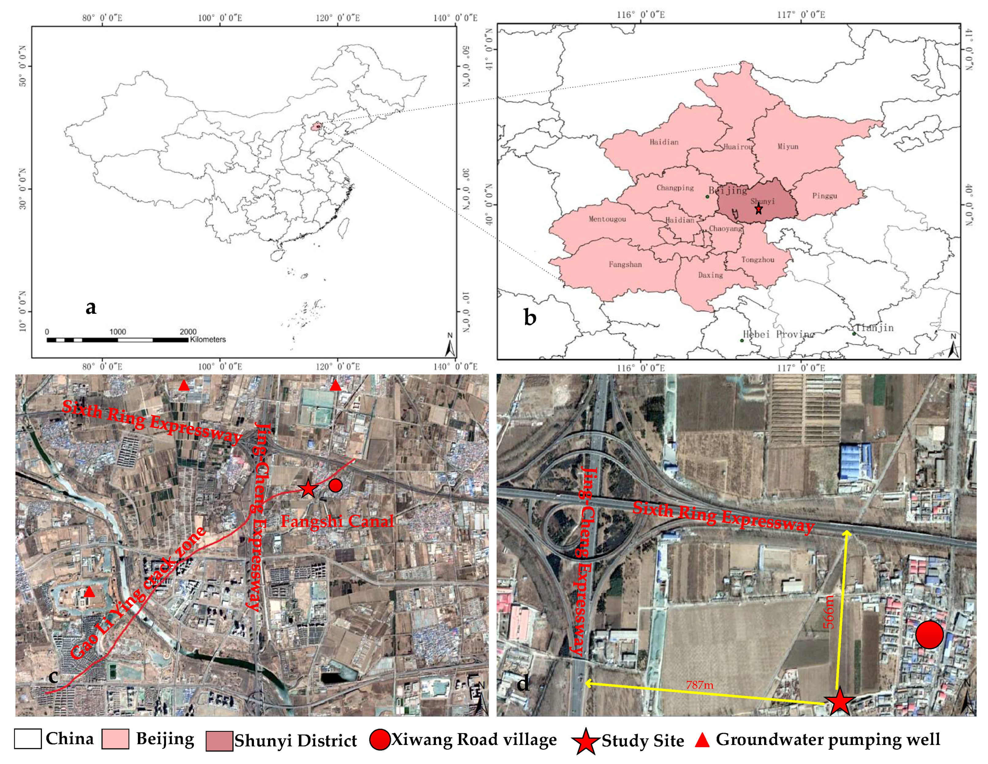
2. Study Site
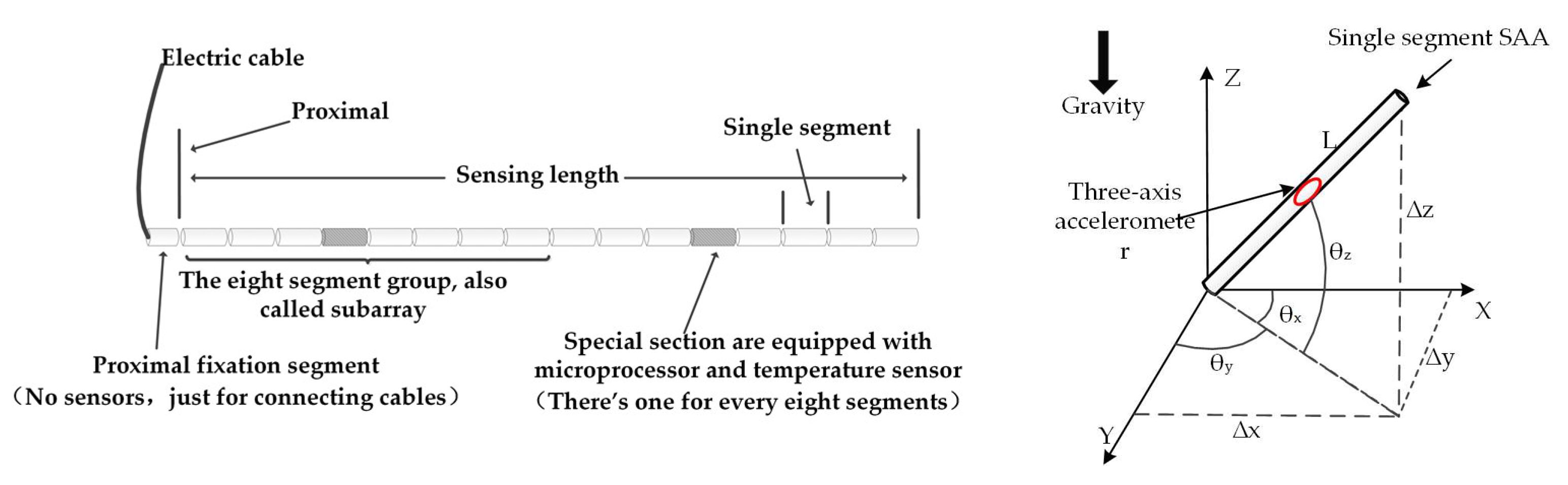
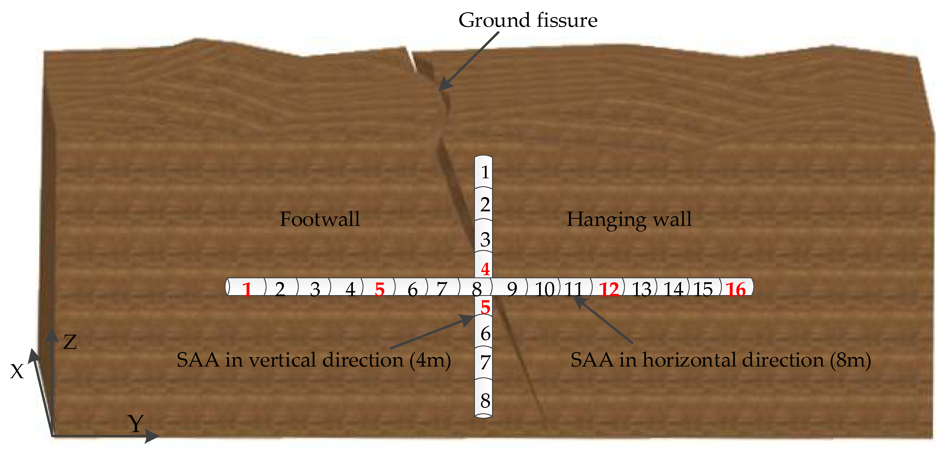
3. SAA Sensor Layout
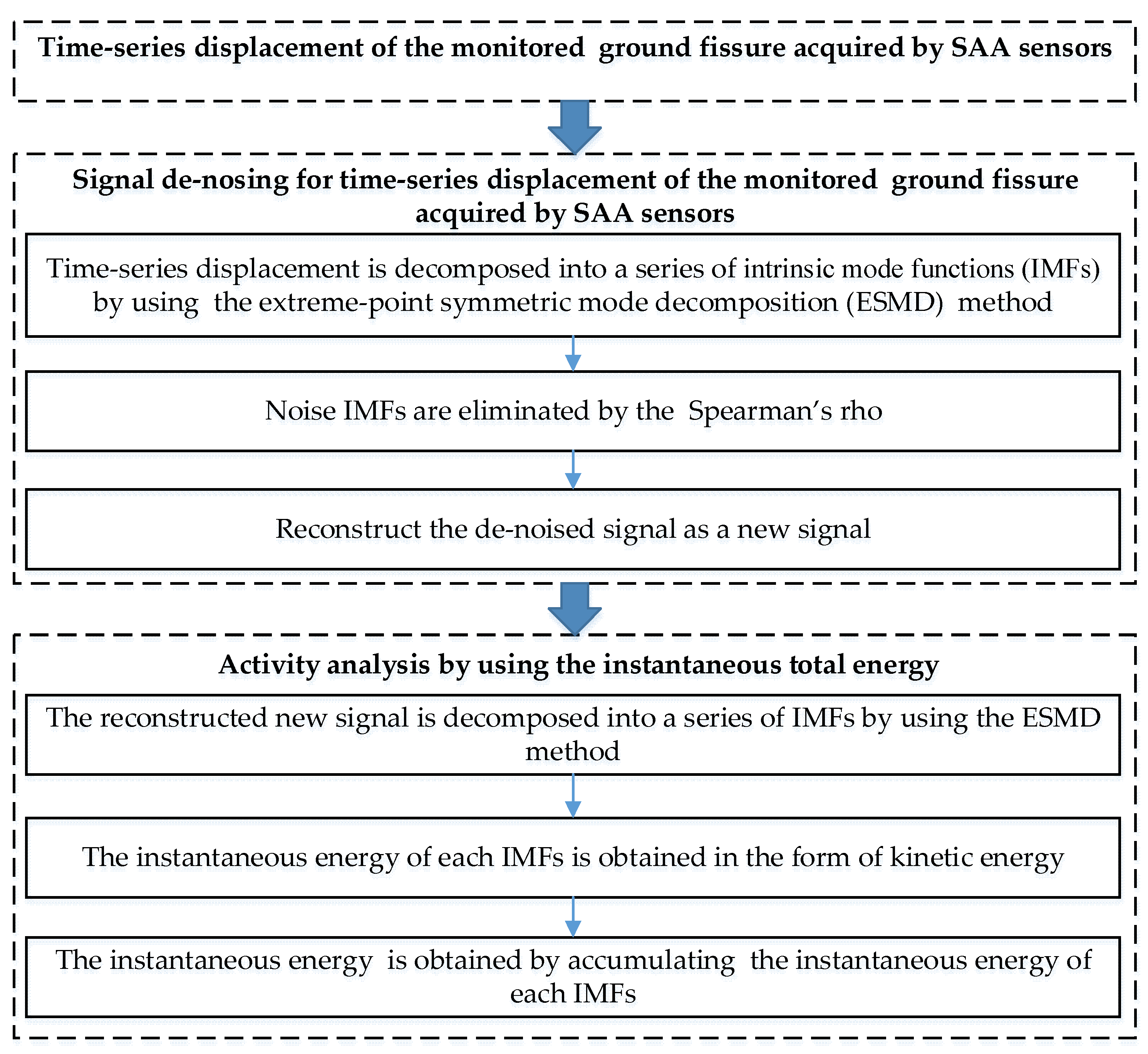
4. Methodology
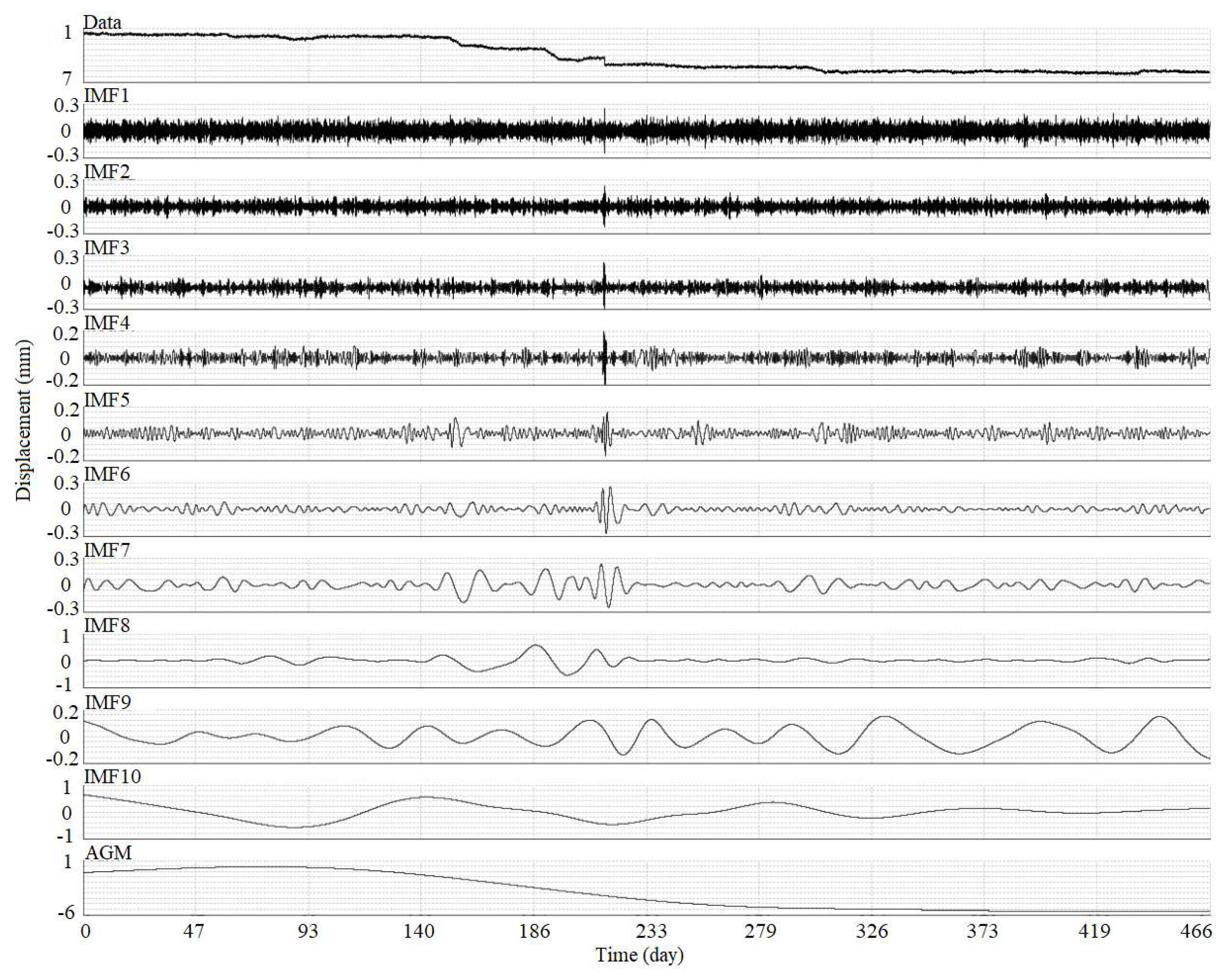
4.1. Signal Denoising Using the ESMD Method and Spearman’s Rho
4.2. Instantaneous Total Energy of the Activity Analysis
5. Results and Discussion
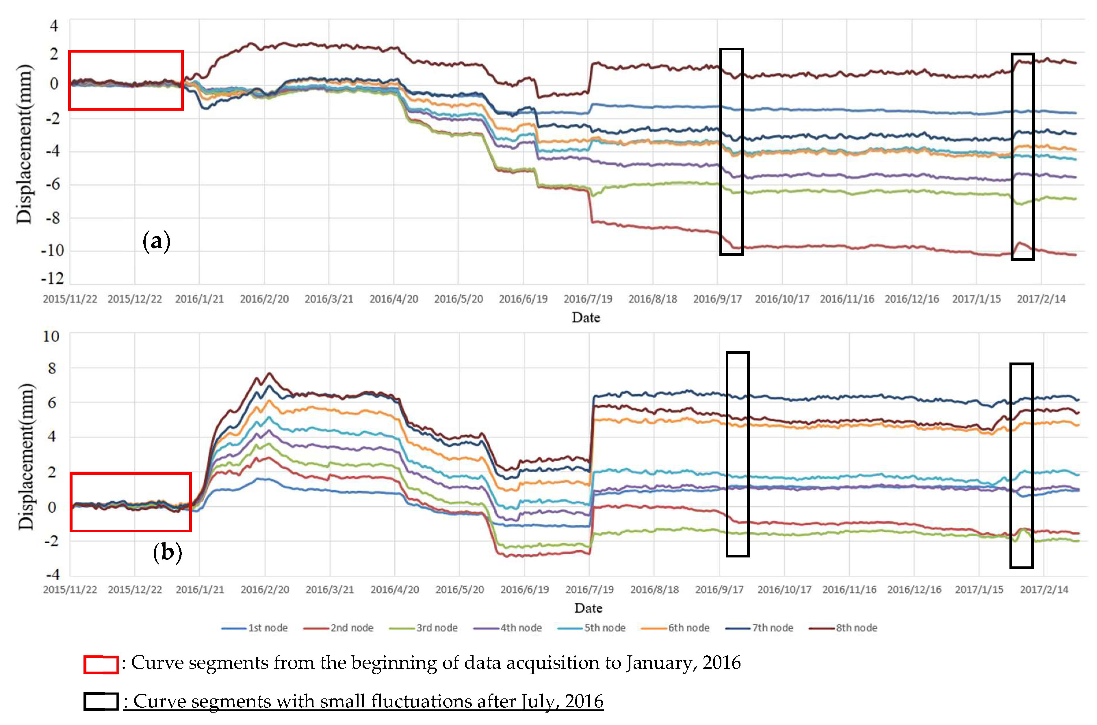
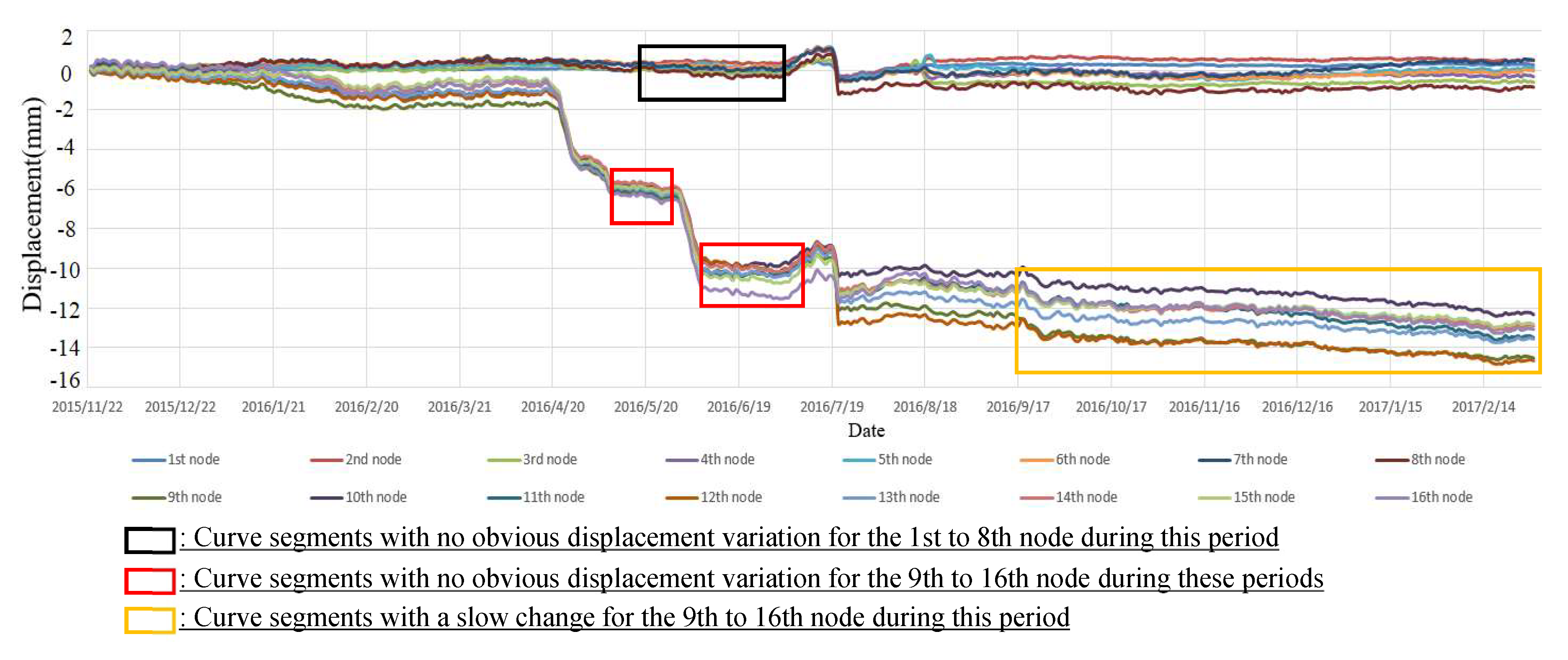
5.1. Results of Variations in the Ground Fissure
5.2. Signal Denoising
5.3. Analysis of Ground Fissure Activity
6. Conclusions
Author Contributions
Funding
Conflicts of Interest
References
- Lee, C.F.; Zhang, J.M.; Zhang, Y.X. Evolution and origin of the ground fissures in Xian, China. Eng. Geol. 1996, 43, 45–55. [Google Scholar] [CrossRef]
- Peng, J.B.; Sun, X.H.; Wang, W. Characteristics of land subsidence, earth fissures and related disaster chain effects with respect to urban hazards in Xi’an, China. Environ. Earth Sci. 2016, 75, 1190. [Google Scholar] [CrossRef]
- Ge, Y.; Tang, H.; Gong, X. Deformation Monitoring of Earth Fissure Hazards Using Terrestrial Laser Scanning. Sensors 2019, 19, 1463. [Google Scholar] [CrossRef] [PubMed]
- Xu, J.; Meng, L.; An, H. The bending mechanism of Anping ground fissure in the Hebei Plain, North China. Environ. Earth Sci. 2015, 74, 6859–6870. [Google Scholar] [CrossRef]
- Qu, F.; Zhang, Q.; Lu, Z.; Zhao, C.; Yang, C.; Zhang, J. Land subsidence and ground fissures in Xi’an, China 2005–2012 revealed by multi-band InSAR time-series analysis. Remote Sens. Environ. 2014, 155, 366–376. [Google Scholar] [CrossRef]
- Desir, G.; Gutiérrez, F.; Merino, J.; Carbonel, D.; Benito-Calvo, A.; Guerrero, J.; Fabregat, I. Rapid subsidence in damaging sinkholes: Measurement by high-precision leveling and the role of salt dissolution. Geomorphology 2018, 303, 393–409. [Google Scholar] [CrossRef]
- Psimoulis, P.; Ghilardi, M.; Fouache, E.; Stiros, S. Subsidence and evolution of the Thessaloniki plain, Greece, based on historical leveling and GPS data. Eng. Geol. 2007, 90, 55–70. [Google Scholar] [CrossRef]
- Zhao, C.Y.; Zhang, Q.; Ding, X.L.; Lu, Z.; Yang, C.S.; Qi, X.M. Monitoring of land subsidence and ground fissures in Xian, China 2005–2006: Mapped by SAR interferometry. Environ. Geol. 2009, 58, 1533–1540. [Google Scholar] [CrossRef]
- Lee, J.; Snyder, P.K.; Fisher, P.F. Modeling the effect of data errors on feature extraction from digital elevation models. Photogramm. Eng. Remote Sens. 1992, 58, 1461. [Google Scholar]
- Bonforte, A.; Guglielmino, F.; Palano, M.; Puglisi, G. A syn-eruptive ground deformation episode measured by GPS, during the 2001 eruption on the upper southern flank of Mt Etna. Bull. Volcanol. 2004, 66, 336–341. [Google Scholar] [CrossRef]
- Gili, J.A.; Corominas, J.; Rius, J. Using Global Positioning System techniques in landslide monitoring. Eng. Geol. 2000, 55, 167–192. [Google Scholar] [CrossRef]
- Qu, W.; Lu, Z.; Zhang, Q. Kinematic model of crustal deformation of Fenwei basin, China based on GPS observations. J. Geodyn. 2014, 75, 1–8. [Google Scholar] [CrossRef]
- Massonnet, D.; Rossi, M.; Carmona, C. The displacement field of the Landers earthquake mapped by radar interferometry. Nature 1993, 364, 138–142. [Google Scholar] [CrossRef]
- Lu, Z.; Fielding, E.; Patrick, M.R. Estimating lava volume by precision combination of multiple baseline spaceborne and airborne interferometric synthetic aperture radar: The 1997 eruption of Okmok volcano, Alaska. IEEE Trans. Geosci. Remote Sens. 2003, 41, 1428–1436. [Google Scholar]
- Brunori, C.; Bignami, C.; Albano, M.; Zucca, F.; Samsonov, S.; Groppelli, G.; Stramondo, S. Land subsidence, ground fissures and buried faults: InSAR monitoring of Ciudad Guzmán (Jalisco, Mexico). Remote Sens. 2015, 7, 8610–8630. [Google Scholar] [CrossRef]
- Yang, C.; Lu, Z.; Zhang, Q.; Liu, R.; Ji, L.; Zhao, C. Ground deformation and fissure activity in Datong basin, China 2007–2010 revealed by multi-track InSAR. Geomat. Nat. Haz. Risk 2019, 10, 465–482. [Google Scholar] [CrossRef]
- Bonforte, A.; Ferretti, A.; Prati, C. Calibration of atmospheric effects on SAR interferograms by GPS and local atmosphere models: First results. J. Atmos. Sol.-Terr. Phys. 2001, 63, 1343–1357. [Google Scholar] [CrossRef]
- Suo, W.; Lu, Y.; Shi, B.; Zhu, H.; Wei, G.; Jiang, H. Evelopment and application of a fixed-point fiber-optic sensing cable for ground fissure monitoring. J. Civ. Struct. Health Monit. 2016, 6, 715–724. [Google Scholar] [CrossRef]
- Ye, S.; Xue, Y.; Wu, J.; Yan, X.; Yu, J. Progression and mitigation of land subsidence in China. Hydrogeol. J. 2016, 24, 685–693. [Google Scholar] [CrossRef]
- Zhu, H.H.; Shi, B.; Zhang, C.C. FBG-based monitoring of geohazards: Current status and trends. Sensors 2017, 17, 452. [Google Scholar] [CrossRef]
- Amoruso, A.; Crescentini, L.; Scarpa, R.; Bilham, R.; Linde, A.T.; Sacks, I.S. Abrupt magma chamber contraction and microseismicity at Campi Flegrei, Italy: Cause and effect determined from strainmeters and tiltmeters. J. Geophys. Res. 2015, 120, 5467–5478. [Google Scholar] [CrossRef]
- Bradley, B.; Prado, G.R. The Use of Shape Accel Array for Monitoring Utilities during Urban Tunnel Drives. In Crossrail Project: Infrastructure Design and Construction; ICE Publishing: London, UK, 2015; pp. 221–237. [Google Scholar]
- Uhlemann, S.; Smith, A.; Chambers, J. Assessment of ground-based monitoring techniques applied to landslide investigations. Geomorphology 2016, 253, 438–451. [Google Scholar] [CrossRef]
- Buchli, T.; Laue, J.; Springman, S.M. Amendments to interpretations of SAAF inclinometer data from the Furggwanghorn rock glacier, Turtmann Valley, Switzerland: Results from 2010 to 2012. Vadose Zone J. 2016, 15. [Google Scholar] [CrossRef]
- Abdoun, T.; Bennett, V.; Danisch, L. Real-Time Construction Monitoring with a Wireless Shape-Acceleration Array System. Geotech. Spec. Publ. 2008, 179, 533–540. [Google Scholar]
- Macciotta, R.; Hendry, M.; Martin, C.D. Developing an early warning system for a very slow landslide based on displacement monitoring. Nat. Hazard 2015, 81, 1–21. [Google Scholar] [CrossRef]
- Dijkstra, T.A.; Dixon, N. Climate change and slope stability in the UK: Challenges and approaches. Q. J. Eng. Geol. Hydrogeol. 2010, 43, 371–385. [Google Scholar] [CrossRef]
- Huntley, D.; Bobrowsky, P.; Qing, Z.; Sladen, W.; Bunce, C.; Edwards, T.; Choi, E. Fiber optic strain monitoring and evaluation of a slow-moving landslide near Ashcroft, British Columbia, Canada. In Landslide Science for a Safer Geoenvironment; Springer International Publishing: New York, NY, USA, 2014; pp. 415–421. [Google Scholar]
- Journault, J.; Macciotta, R.; Hendry, M.T.; Charbonneau, F.; Huntley, D.; Bobrowsky, P.T. Measuring displacements of the Thompson River valley landslides, south of Ashcroft, BC, Canada, using satellite InSAR. Landslides 2018, 15, 621–636. [Google Scholar] [CrossRef]
- Chang, P.Y.; Huang, W.J.; Chen, C.C.; Hsu, H.L.; Yen, I.C.; Ho, G.R.; Chen, P.T. Probing the frontal deformation zone of the Chihshang Fault with boreholes and high-resolution electrical resistivity imaging methods: A case study at the Dapo site in eastern Taiwan. J. Appl. Geophys. 2018, 153, 127–135. [Google Scholar] [CrossRef]
- Yang, C.; Zhang, Q.; Zhao, C.; Ji, L. Small Baseline Bubset InSAR Technology Used in Datong Basin Ground Subsidence, Fissure and Fault Zone Monitoring. Geomat. Inf. Sci. Wuhan Univ. 2014, 39, 945–950. (In Chinese) [Google Scholar]
- Cheng, G.; Wang, H.; Luo, Y. Study of the deformation mechanism of the Gaoliying ground fissure. Proc. IAHS 2015, 372, 231–234. [Google Scholar] [CrossRef][Green Version]
- Huang, N.E.; Shen, Z.; Long, S.R. The Empirical Mode Decomposition and the Hilbert Spectrum for Nonlinear and Non-Stationary Time Series Analysis. Proc. R. Soc. A 1998, 454, 903–995. [Google Scholar] [CrossRef]
- Liu, X.; Lu, Z.; Yang, W. Dynamic Monitoring and Vibration Analysis of Ancient Bridges by Ground-Based Microwave Interferometry and the ESMD Method. Remote Sens. 2018, 10, 770. [Google Scholar] [CrossRef]
- Kopsinis, Y.; Mclaughlin, S. Development of EMD-based denoising methods inspired by wavelet thresholding. IEEE Trans. Signal Process. 2009, 57, 1351–1362. [Google Scholar] [CrossRef]
- Gan, Y.; Sui, L.; Wu, J. An EMD threshold de-noising method for inertial sensors. Measurement 2014, 49, 34–41. [Google Scholar] [CrossRef]
- Wang, J.L.; Li, Z.J. Extreme-point symmetric mode decomposition method for data analysis. Adv. Adapt. Data Anal. 2013, 5, 1350015. [Google Scholar] [CrossRef]
- Schreier, P. A unifying discussion of correlation analysis for complex random vectors. IEEE Trans. Signal Process. 2008, 56, 1327–1336. [Google Scholar] [CrossRef]
- Xu, W.C. A comparative analysis of Spearman’s rho and Kendall’s tau in normal and contaminated normal models. Signal Process. 2013, 93, 261–276. [Google Scholar] [CrossRef]
- Duan, Y.B.; Song, C.T. Relevant modes selection method based on Spearman correlation coefficient for laser signal denoising using empirical mode decomposition. Opt. Rev. 2016, 23, 936–949. [Google Scholar] [CrossRef]
- Li, J.W. A UV-visible absorption spectrum denoising method based on EEMD and an improved universal threshold filter. RSC Adv. 2018, 8, 8558–8568. [Google Scholar] [CrossRef]
- Huang, N.E.; Chen, X.; Lo, M.T.; Wu, Z. On Hilbert spectral representation: A true time-frequency representation for nonlinear and nonstationary data. Adv. Adapt. Data Anal. 2011, 3, 63–93. [Google Scholar] [CrossRef]
- Si, L.; Wang, Q. Rapid multi-damage identification for health monitoring of laminated composites using piezoelectric wafer sensor arrays. Sensors 2016, 16, 638. [Google Scholar] [CrossRef] [PubMed]
- Liu, X.; Tang, Y.; Lu, Z.; Huang, H.; Tong, X.; Ma, J. ESMD-based stability analysis in the progressive collapse of a building model: A case study of a reinforced concrete frame-shear wall model. Measurement 2018, 120, 34–42. [Google Scholar] [CrossRef]


© 2019 by the authors. Licensee MDPI, Basel, Switzerland. This article is an open access article distributed under the terms and conditions of the Creative Commons Attribution (CC BY) license (http://creativecommons.org/licenses/by/4.0/).
Share and Cite
Liu, X.; Su, S.; Ma, J.; Yang, W. Deformation Activity Analysis of a Ground Fissure Based on Instantaneous Total Energy. Sensors 2019, 19, 2607. https://doi.org/10.3390/s19112607
Liu X, Su S, Ma J, Yang W. Deformation Activity Analysis of a Ground Fissure Based on Instantaneous Total Energy. Sensors. 2019; 19(11):2607. https://doi.org/10.3390/s19112607
Chicago/Turabian StyleLiu, Xianglei, Shan Su, Jing Ma, and Wanxin Yang. 2019. "Deformation Activity Analysis of a Ground Fissure Based on Instantaneous Total Energy" Sensors 19, no. 11: 2607. https://doi.org/10.3390/s19112607
APA StyleLiu, X., Su, S., Ma, J., & Yang, W. (2019). Deformation Activity Analysis of a Ground Fissure Based on Instantaneous Total Energy. Sensors, 19(11), 2607. https://doi.org/10.3390/s19112607