An Affinity Propagation-Based Self-Adaptive Clustering Method for Wireless Sensor Networks


Abstract
:1. Introduction
2. Related Work
3. System Model
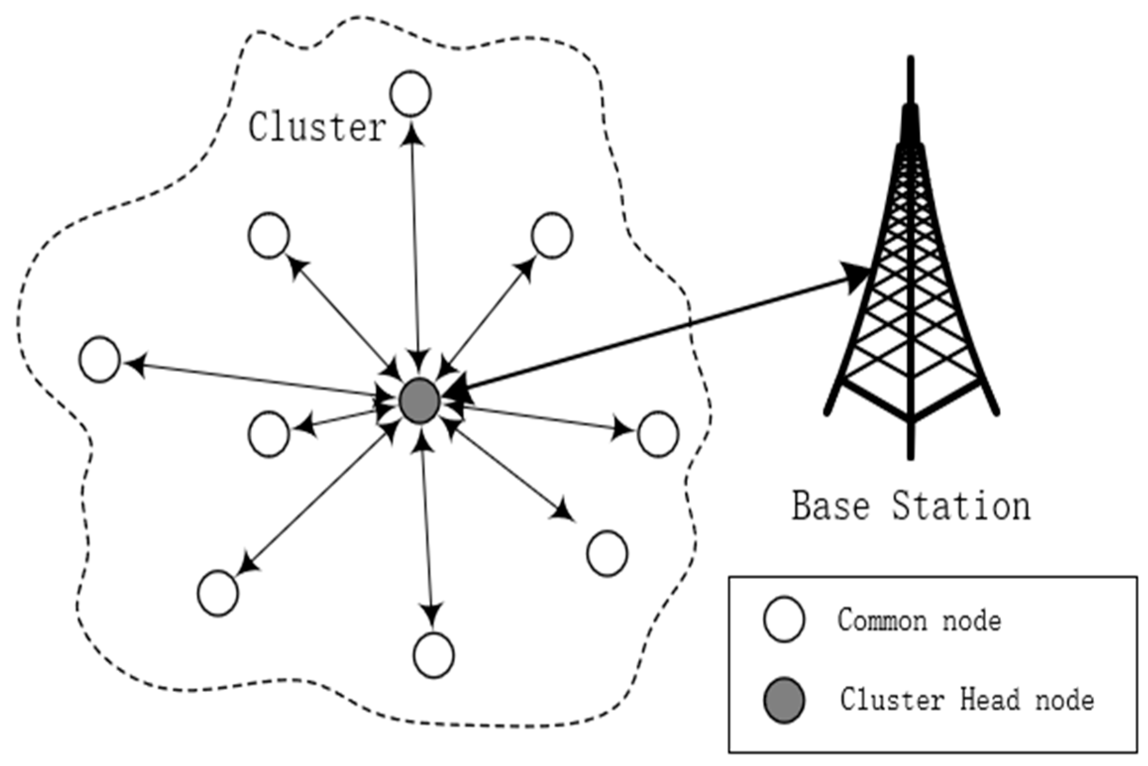
3.1. Network Model
- All the sensors are deployed in a rectangle area by planes or other vehicles and they keep stationary after they are deployed.
- Sensor nodes can be identified by their unique ID.
- Each sensor owns the knowledge of its position by the equipment such as the Global Positioning System (GPS), and they can get the information of other nodes by information exchange.
- All the sensors own the same initial energy and their batteries cannot be changed. Once they exhaust their energy, they will be useless.
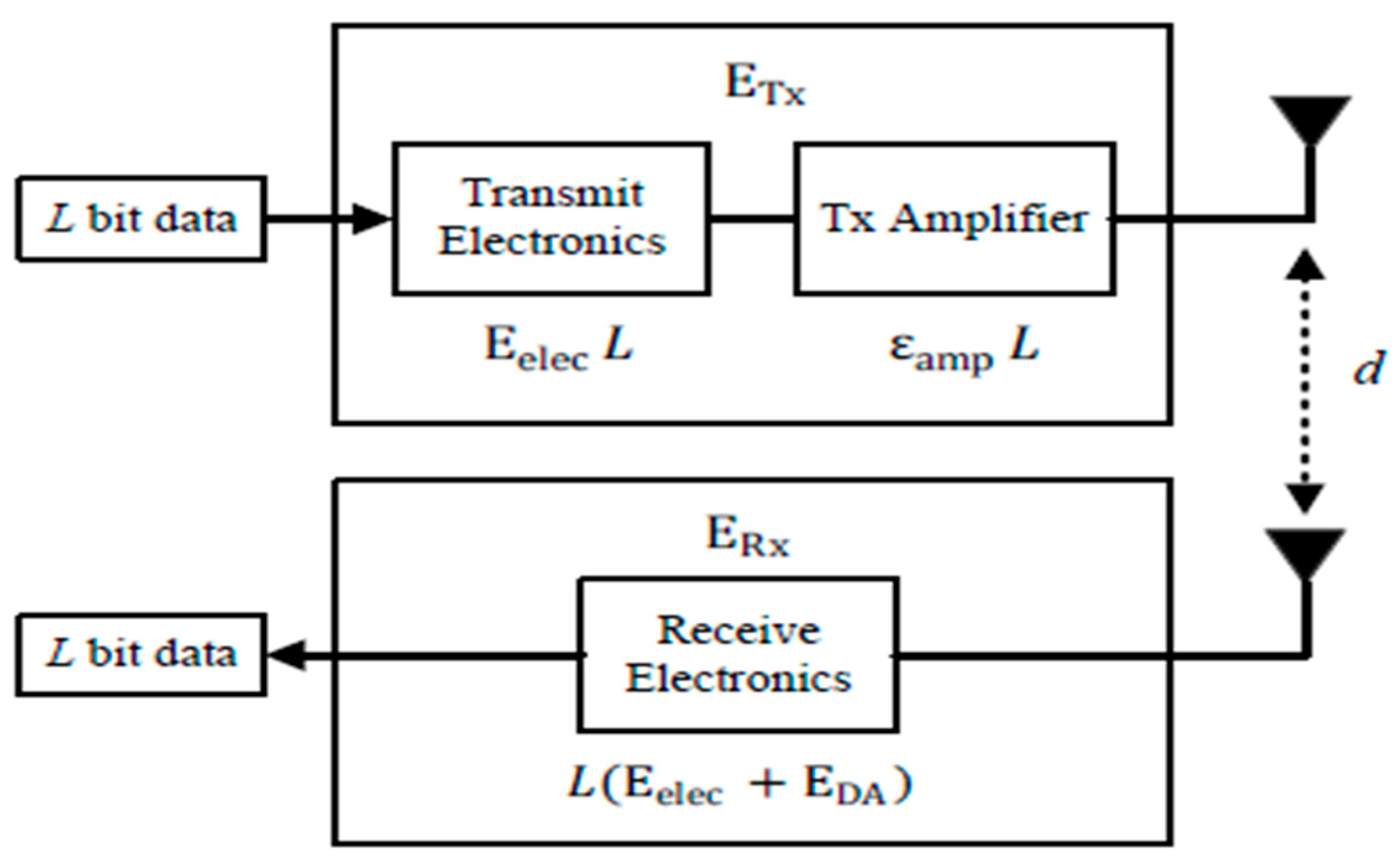
3.2. Energy Model
4. The Proposed Affinity Propagation-Based Self-Adaptive (APSA) Algorithm
4.1. Initial Phase
4.2. Set-Up Phase
| Algorithm 1: The method for obtaining initial cluster centers |
| Input: the coordinate set of N sensor nodes ; |
| fori = 1, 2, 3, …, Ndo |
| for j = 1, 2, 3, …, N do |
| if i == j then |
| set preference |
| else |
| calculate similarity |
| end if |
| end for |
| end for |
| Repeat |
| for i = 1, 2, 3, …, N |
| for j = 1, 2, 3, …, N |
| calculate responsibility |
| if i == j then |
| else |
| end if |
| calculate |
| End for |
| End for |
| UntilT does not change |
| Algorithm 2: The method for clustering |
| let T as the set of initial cluster centers; |
| calculate the number of initial cluster centers |
| Repeat |
| assign each remaining common node to the cluster with the nearest medoid; |
| randomly select a common sensor node ; |
| calculate the cost function of swapping node with ; |
| if S<0 then |
| swap with to form the new set of k clusters; |
| Until no change |
| Output: a set of k clusters. |
4.3. Communication Phase
5. Performance Evaluation
5.1. Simulation Parameters
5.2. Clustering Results of Different Number of Sensors
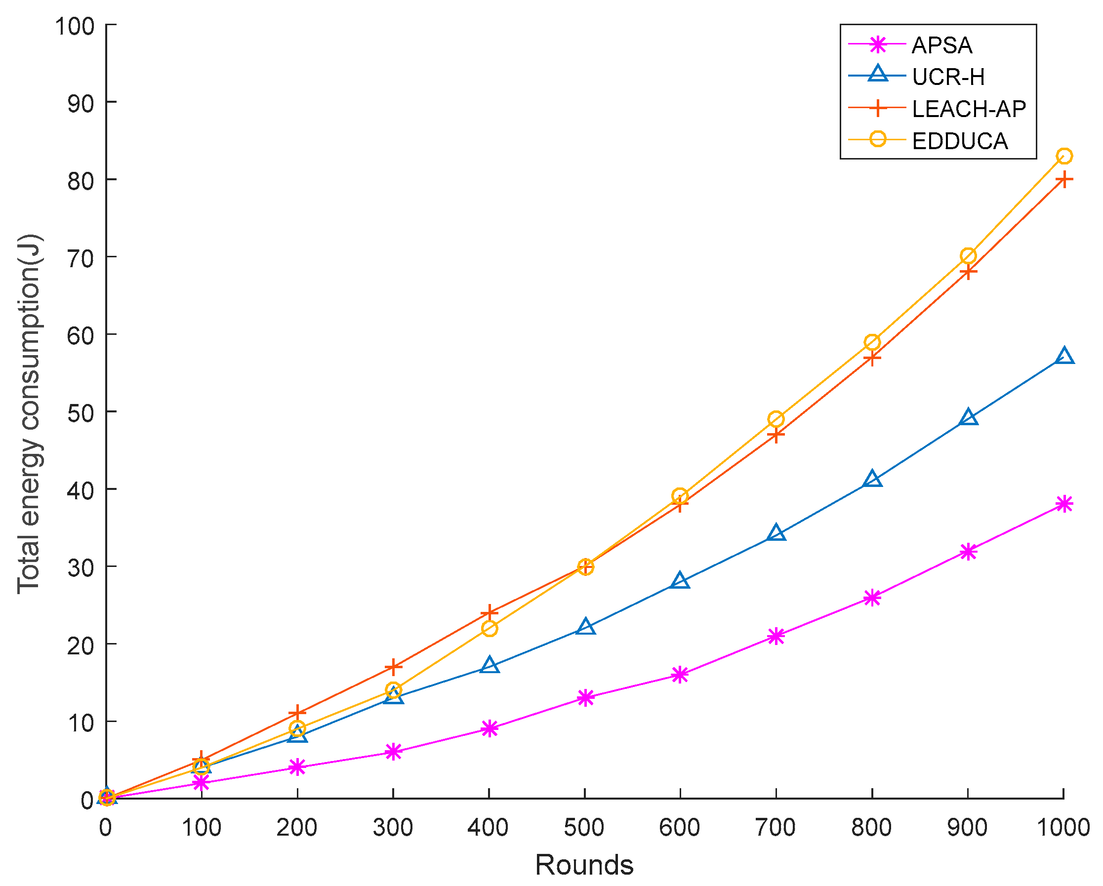
5.3. Analysis of Energy Consumption
5.4. Analysis of Network Lifetime
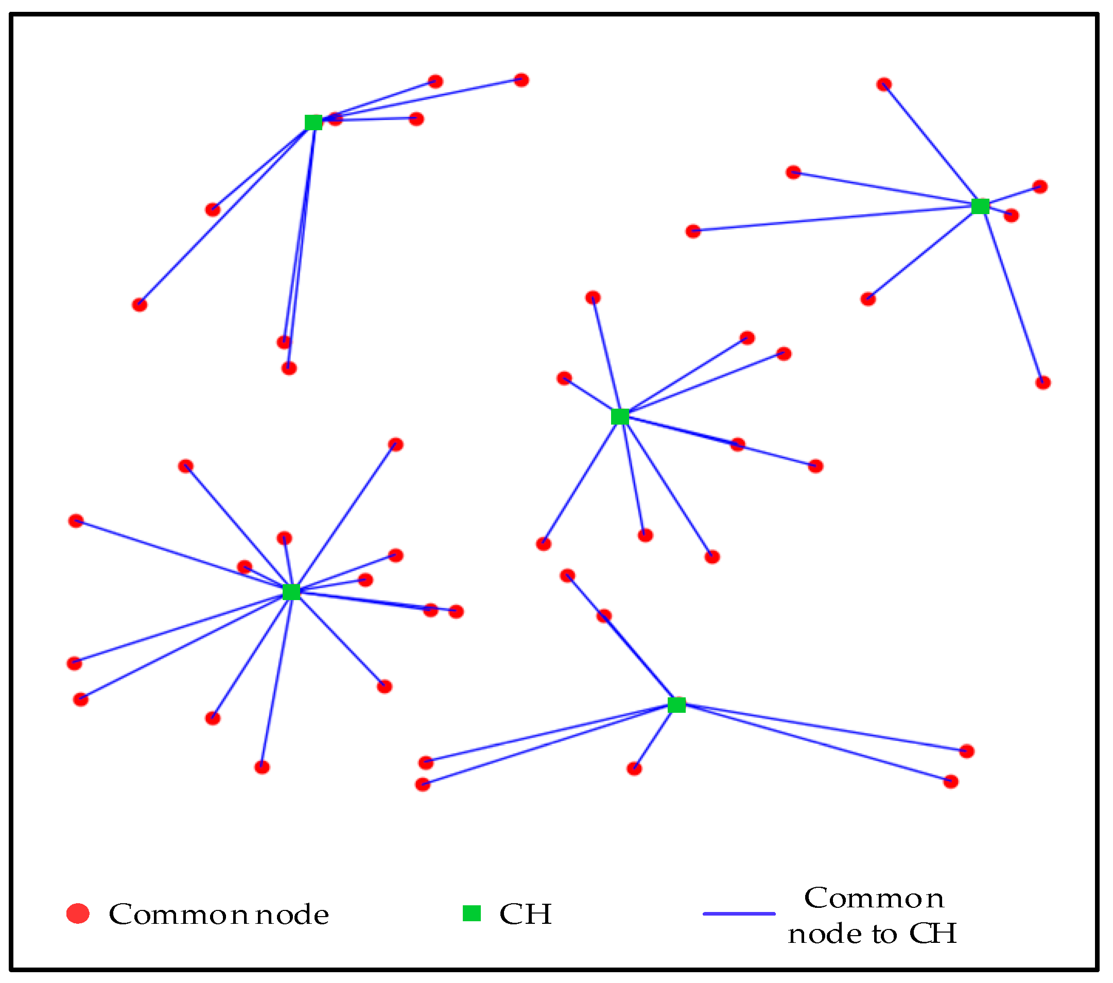
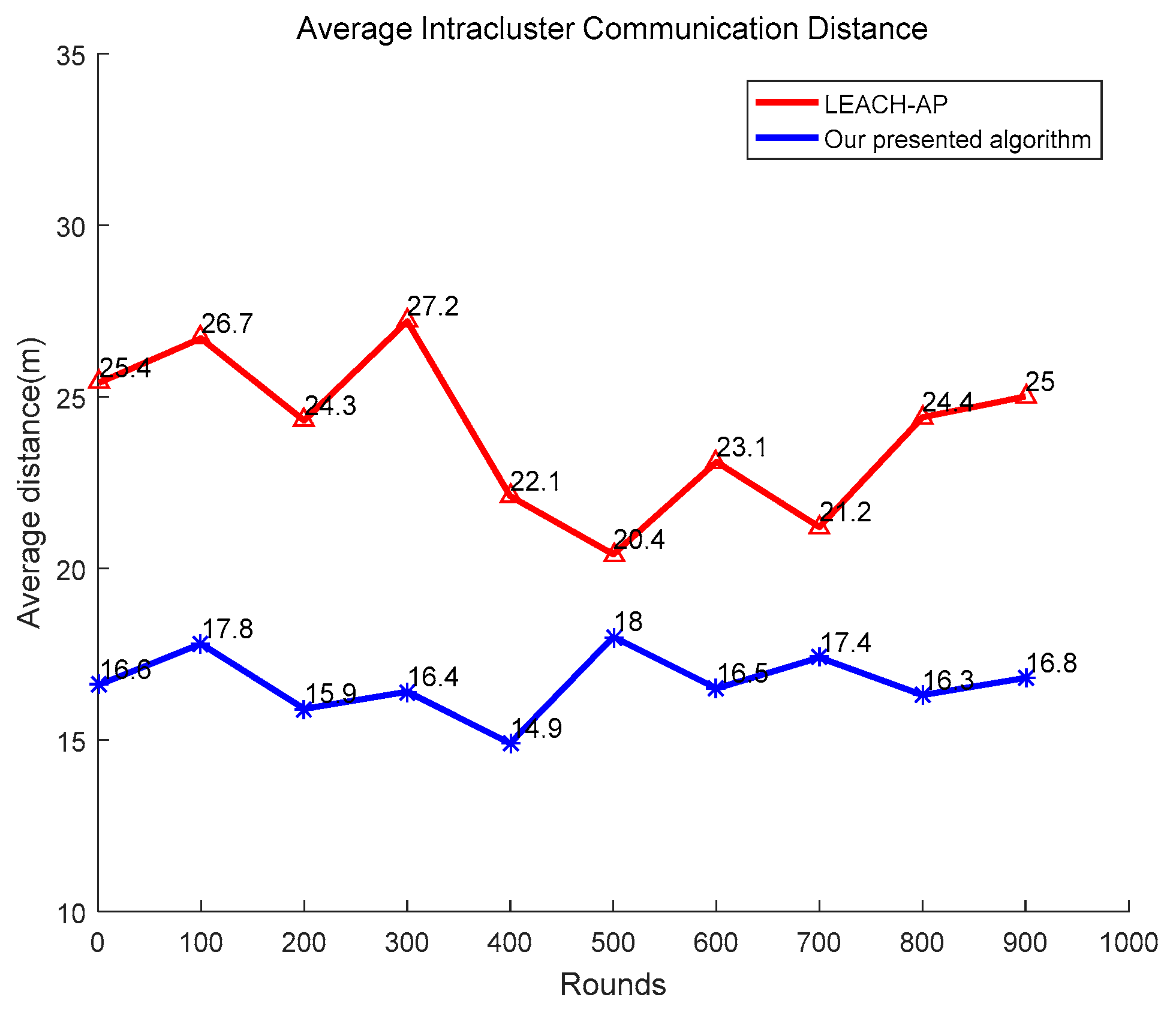
5.5. Analysis of Clustering Result
5.6. Study of Affinity Propagation (AP) Preference
6. Discussion
7. Conclusions
Author Contributions
Acknowledgments
Conflicts of Interest
Data Availability
References
- Potdar, V.; Sharif, A.; Chang, E. Wireless Sensor Networks: A Survey. Comput. Netw. 2002, 38, 393–422. [Google Scholar]
- Wang, J.; Gao, Y.; Liu, W.; Sangaiah, A.K.; Kim, H. An Intelligent Data Gathering Schema with Data Fusion Supported for Mobile Sink in WSNs. Int. J. Distrib. Sens. Netw. 2019, 15. [Google Scholar] [CrossRef]
- Yue, Y.G.; He, P. A comprehensive survey on the reliability of mobile wireless sensor networks: Taxonomy, challenges, and future directions. Inf. Fusion 2018, 44, 188–204. [Google Scholar] [CrossRef]
- Wang, J.; Gao, Y.; Liu, W.; Sangaiah, A.K.; Kim, H. Energy Efficient Routing Algorithm with Mobile Sink Support for Wireless Sensor Networks. Sensors 2019, 19, 2363. [Google Scholar] [CrossRef] [PubMed]
- Al-Karaki, J.N.; Kamal, A.E. Routing techniques in wireless sensor networks: A survey. IEEE Wirel. Commun. 2004, 11, 6–28. [Google Scholar] [CrossRef]
- Wang, J.; Ju, C.; Gao, Y.; Sangaiah, A.K.; Kim, G. A PSO based Energy Efficient Coverage Control Algorithm for Wireless Sensor Networks. Comput. Mater. Contin. 2018, 56, 433–446. [Google Scholar]
- Imon, S.K.A.; Khan, A.; Francesco, M.D. Energy-efficient randomized switching for maximizing lifetime in tree-based wireless sensor networks. IEEE ACM Trans. Netw. 2015, 23, 1401–1415. [Google Scholar] [CrossRef]
- Wang, J.; Zhang, Z.; Li, B.; Lee, S.Y.; Sherratt, R.S. An Enhanced Fall Detection System for Elderly Person Monitoring using Consumer Home Networks. IEEE Trans. Consum. Electron. 2014, 60, 23–29. [Google Scholar] [CrossRef]
- Wang, J.; Cao, J.; Sherratt, R.S.; Park, J.H. An improved ant colony optimization-based approach with mobile sink for wireless sensor networks. J. Supercomput. 2018, 74, 6633–6645. [Google Scholar] [CrossRef]
- Arain, Q.A.; Uqaili, M.A.; Deng, Z. Clustering Based Energy Efficient and Communication Protocol for Multiple Mix-Zones Over Road Networks. Wirel. Pers. Commun. 2016, 95, 411–428. [Google Scholar] [CrossRef]
- Wang, J.; Gao, Y.; Yin, X.; Li, F.; Kim, H. An Enhanced PEGASIS Algorithm with Mobile Sink Support for Wireless Sensor Networks. Wirel. Commun. Mob. Comput. 2018, 9472075. [Google Scholar] [CrossRef]
- Wang, F.; Wu, S.; Wang, K. Energy-Efficient Clustering Using Correlation and Random Update Based on Data Change Rate for Wireless Sensor Networks. IEEE Sens. J. 2016, 16, 5471–5480. [Google Scholar] [CrossRef]
- Ya, T.; Lin, Y.; Wang, J.; Kim, J. Semi-supervised Learning with Generative Adversarial Networks on Digital Signal Modulation Classification. Comput. Mater. Contin. 2018, 55, 243–254. [Google Scholar]
- Wang, J.; Gao, Y.; Liu, W.; Wu, W.; Lim, S. An Asynchronous Clustering and Mobile Data Gathering Schema based on Timer Mechanism in Wireless Sensor Networks. Comput. Mater. Contin. 2019, 58, 711–725. [Google Scholar] [CrossRef]
- Heinzelman, W.; Chandrakasan, A.; Balakrishnan, H. Energy-efficient communication protocol for wireless microsensor networks. In Proceedings of the Hawaii International Conference on System Sciences, Big Island, HI, USA, 7–10 January 2002; p. 8020. [Google Scholar]
- Lindsey, S. PEGASIS: Power-efficient gathering in sensor information system. In Proceedings of the IEEE Aerospace Conference, Big Sky, MT, USA, 9–16 March 2002; Volume 3, pp. 1125–1130. [Google Scholar]
- Kaufman, L.; Rousseeuw, P.A. Clustering by Means of Medoids.Statistical Data Analysis Based on the L 1 Norm; Elsevier: Berlin, Germany, 1987; pp. 405–416. [Google Scholar]
- Heinzelman, W.B.; Chandrakasan, A.P.; Balakrishnan, H. An application-specific protocol architecture for wireless microsensor networks. IEEE Trans. Wirel. Commun. 2002, 1, 660–670. [Google Scholar] [CrossRef]
- Illsoo, S.; Lee, J.-H.; Lee, S.H. Low-energy adaptive clustering hierarchy using affinity propagation for wireless sensor networks. IEEE Commun. Lett. 2016, 20, 558–561. [Google Scholar]
- Younis, O.; Fahmy, S. HEED: A Hybrid, Energy-efficient, Distributed Clustering Approach for Ad hoc Sensor Networks. IEEE Trans. Mob. Comput. 2004, 3, 366–379. [Google Scholar] [CrossRef]
- Manjeshwar, A.; Agrawal, D.P. TEEN: A Routing Protocol for Enhanced Efficiency in Wireless Sensor Networks. In Proceedings of the International Parallel and Distributed Processing Symposium, San Francisco, CA, USA, 23–27 April 2000. [Google Scholar]
- Chang, J.Y.; Ju, P.H. An efficient cluster-based power saving scheme for wireless sensor networks. Eurasip J. Wirel. Commun. Netw. 2012, 1–10. [Google Scholar] [CrossRef]
- Bagci, H.; Yazici, A. An energy aware fuzzy unequal clustering algorithm for wireless sensor networks. In Proceedings of the 2010 IEEE International Conference on Fuzzy Systems, Barcelona, Spain, 18–23 July 2010. [Google Scholar]
- Li, C.; Ye, M.; Chen, G. An energy-efficient unequal clustering mechanism for wireless sensor networks. In Proceedings of the IEEE International Conference on Mobile Adhoc and Sensor Systems Conference, Washington, DC, USA, 7 November 2005. [Google Scholar]
- Yang, L.; Lu, Y.Z.; Zhong, Y.C. An unequal cluster-based routing scheme for multi-level heterogeneous wireless sensor networks. Telecommun. Syst. 2017, 68, 1–16. [Google Scholar] [CrossRef]
- Guiloufi, A.B.F.; Nasri, N.; Kachouri, A. An Energy-Efficient Unequal Clustering Algorithm Using ‘Sierpinski Triangle’ for WSNs. Wirel. Pers. Commun. 2016, 88, 449–465. [Google Scholar] [CrossRef]
- Wang, J.; Gao, Y.; Liu, W.; Sangaiah, A.K.; Kim, H. An Improved Routing Schema with Special Clustering using PSO Algorithm for Heterogeneous Wireless Sensor Network. Sensors 2019, 19, 671. [Google Scholar] [CrossRef] [PubMed]
- Neamatollahi, P.; Naghibzadeh, M.; Abrishami, S. Fuzzy-Based Clustering-Task Scheduling for Lifetime Enhancement in Wireless Sensor Networks. IEEE Sens. J. 2017, 17, 6837–6844. [Google Scholar] [CrossRef]
- Afsar, M.; Tayarani-N, M.H. Clustering in sensor networks: A literature survey. J. Netw. Comput. Appl. 2014, 46, 198–226. [Google Scholar] [CrossRef]
- Wang, J.; Cao, J.; Ji, S.; Park, J.H. Energy Efficient Cluster-based Dynamic Routes Adjustment Approach for Wireless Sensor Networks with Mobile Sinks. J. Supercomput. 2017, 73, 3277–3290. [Google Scholar] [CrossRef]


| Algorithm Name | Year | Structure | CH Election Features | Topology Control | Methods Used | Demerit |
|---|---|---|---|---|---|---|
| LEACH | 2002 | Two-layer structure | Random selection | Distributed | Uneven CH distribution | |
| LEACH-C | 2002 | Two-layer structure | Residual energy, position | Centralized | High energy consumption | |
| LEACH-AP | 2016 | Two-layer structure | position | Centralized | AP algorithm | Number of clusters assigning |
| PEGASIS | 2002 | Chain-structure | Position | Distributed | Greedy algorithm | Heavy network latency, poor robustness |
| HEED | 2004 | Two-layer structure | position | Distributed | Iteration | Long iteration time |
| TEEN | 2001 | Two-layer structure | Residual energy, position | Distributed | Iteration | Long iteration time |
| SECA | 2012 | Two-layer structure | Residual energy | Centralized | K-means algorithm | Unreason CHs selection |
| EAUC | 2010 | Two-layer structure | Residual energy, Position, number of neighbors | Centralized | Fuzzy logic system | High energy consumption |
| EEUC | 2005 | Two-layer structure | Residual energy, Position | Distributed | Iteration | High energy consumption |
| UCR-H | 2017 | Two-layer structure | Residual energy, Position | Centralized | Multiple CHs in each cluster | High energy consumption |
| EDDUCA | 2016 | Two-layer structure | Position | Centralized | Sierpinski triangle dividing | High energy consumption |
| Parameter | Definition | Value |
|---|---|---|
| N | Number of nodes | 50 |
| coorBs | Coordinate of the base station (BS) | (40,160) |
| PS | Packet Size for one communication | 2000 bits |
| Initial energy of each node | 2J | |
| Energy consumption per bit | ||
| Transmitter amplifier (Free space model) | ||
| Transmitter amplifier (Multi-path model) | ||
| Data aggregation energy | ||
| p | Affinity propagation (AP) preference | −6000 |
| Value of p | −4500 | −5000 | −5500 | −6000 | −6500 | −7000 | −7500 |
| Converge time (s) | 2.12 | 1.54 | 1.22 | 0.99 | 1.13 | 1.27 | 2.46 |
| Cluster number | 8 | 9 | 8 | 6 | 6 | 8 | 9 |
© 2019 by the authors. Licensee MDPI, Basel, Switzerland. This article is an open access article distributed under the terms and conditions of the Creative Commons Attribution (CC BY) license (http://creativecommons.org/licenses/by/4.0/).
Share and Cite
Wang, J.; Gao, Y.; Wang, K.; Sangaiah, A.K.; Lim, S.-J. An Affinity Propagation-Based Self-Adaptive Clustering Method for Wireless Sensor Networks. Sensors 2019, 19, 2579. https://doi.org/10.3390/s19112579
Wang J, Gao Y, Wang K, Sangaiah AK, Lim S-J. An Affinity Propagation-Based Self-Adaptive Clustering Method for Wireless Sensor Networks. Sensors. 2019; 19(11):2579. https://doi.org/10.3390/s19112579
Chicago/Turabian StyleWang, Jin, Yu Gao, Kai Wang, Arun Kumar Sangaiah, and Se-Jung Lim. 2019. "An Affinity Propagation-Based Self-Adaptive Clustering Method for Wireless Sensor Networks" Sensors 19, no. 11: 2579. https://doi.org/10.3390/s19112579
APA StyleWang, J., Gao, Y., Wang, K., Sangaiah, A. K., & Lim, S.-J. (2019). An Affinity Propagation-Based Self-Adaptive Clustering Method for Wireless Sensor Networks. Sensors, 19(11), 2579. https://doi.org/10.3390/s19112579