Wildcard Fields-Based Partitioning for Fast and Scalable Packet Classification in Vehicle-to-Everything


Abstract
:1. Introduction
- First, we propose a new partitioning field selection algorithm that finds the optimal partitioning field using the number of unique matching ranges and the number of wildcards. As far as we know, it is the first approach to use the concept of wildcards based on the matching range of each node, so the algorithm can minimize duplicated rules compared to existing ones.
- Second, we also propose a new partitioning number per field decision algorithm that chooses two partitioning fields through the partitioning field selection algorithm on each node, and finds the number of partitions based on the selected fields to minimize rule duplication. Since it considers only two fields to choose the partitioning number in contrast to existing algorithms using multiple fields, it is fast without the performance degradation.
2. Related Works
2.1. HyperCuts
2.1.1. Partitioning Field Selection
- : Total number of fields in rules.
- : Number of unique matching ranges for the k-th field, where
- : Average number of unique matching ranges.
2.1.2. Partitioning Number Decision
- : Total number of rules in the current node.
- : Number of partitions for the -th field.
- : Space factor.
- : Maximum number of partitions.
2.2. EffiCuts
2.2.1. Tree Splitting
- : Minimum value matching the -th field. e.g., 0 for protocol field.
- : Maximum value matching the -th field. e.g., 255 for protocol field.
- : Minimum value matching the -th field of a given rule.
- : Maximum value matching the -th field of a given rule.
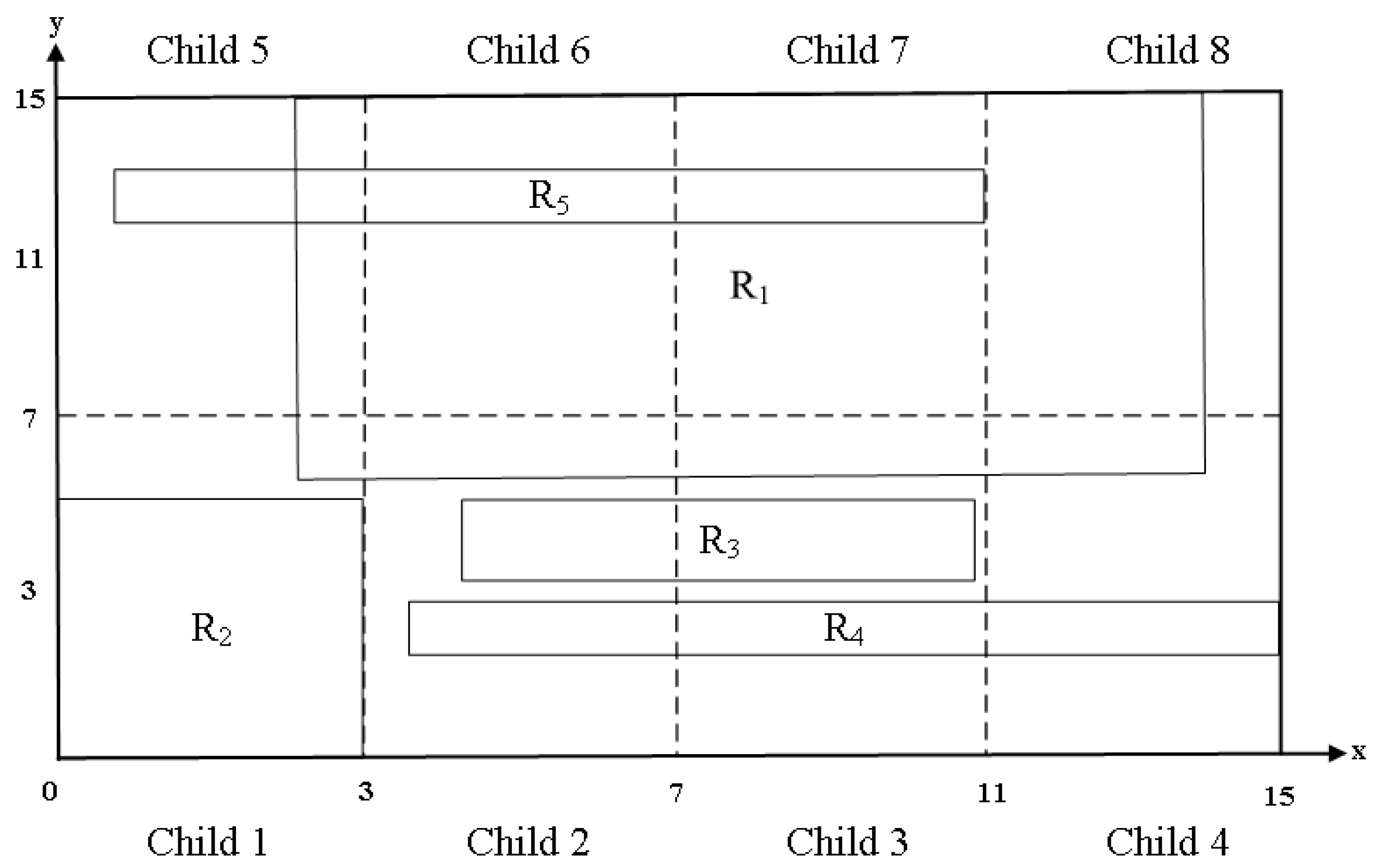
- Category 1: rules with four wildcard fields
- Category 2: rules with three wildcard fields
- Category 3: rules with two wildcard fields
- Category 4: rules with one or zero wildcard field
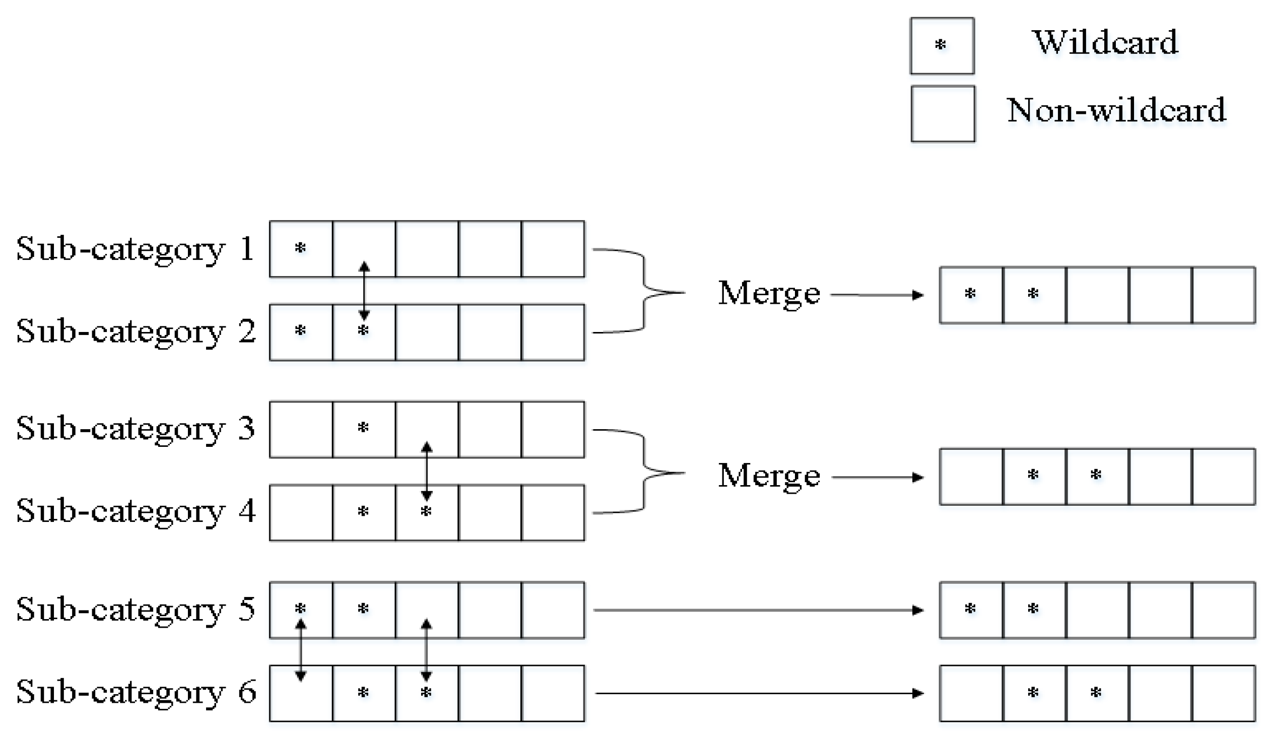
2.2.2. Tree Merging
3. Proposed Algorithm
3.1. Motivation
3.2. Proposed Partitioning Algorithm
3.2.1. Partitioning Field Selection Algorithm
- : The th node.
- : Minimum value matching the -th field at node .
- : -th field at node
- : Minimum value matching the -th field of a given rule at node .
- : Maximum value matching the -th field of a given rule at node .
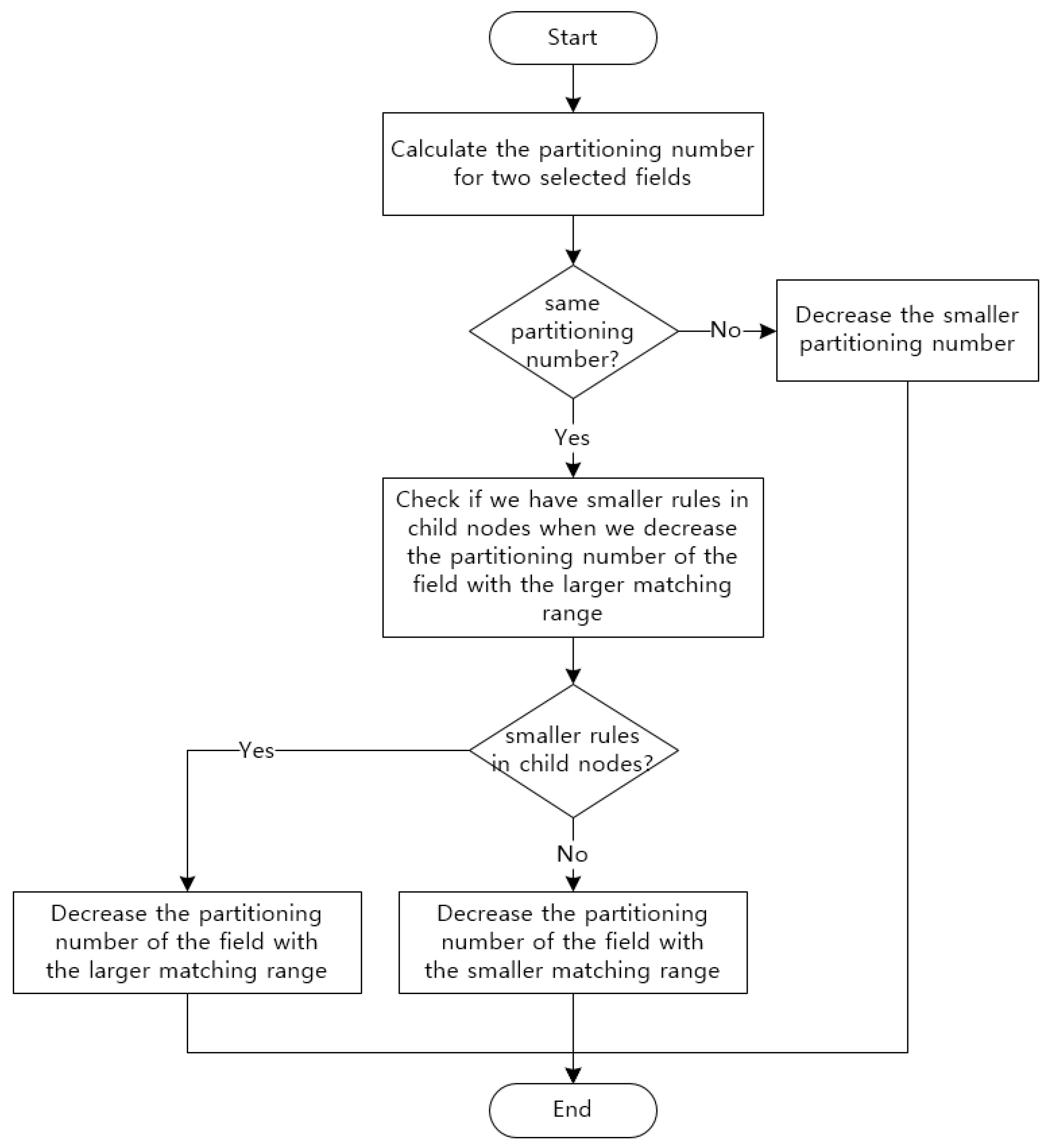
3.2.2. Partitioning Number per Field Decision Algorithm
3.3. Features of the Proposed Algorithm
3.3.1. High Flexibility
3.3.2. Low Memory Requirement
3.3.3. Fast Decision Tree Building Speed
3.3.4. Improved Classification Performance due to Memory Reduction
4. Performance Evaluation
4.1. Memory Requirement per Rule
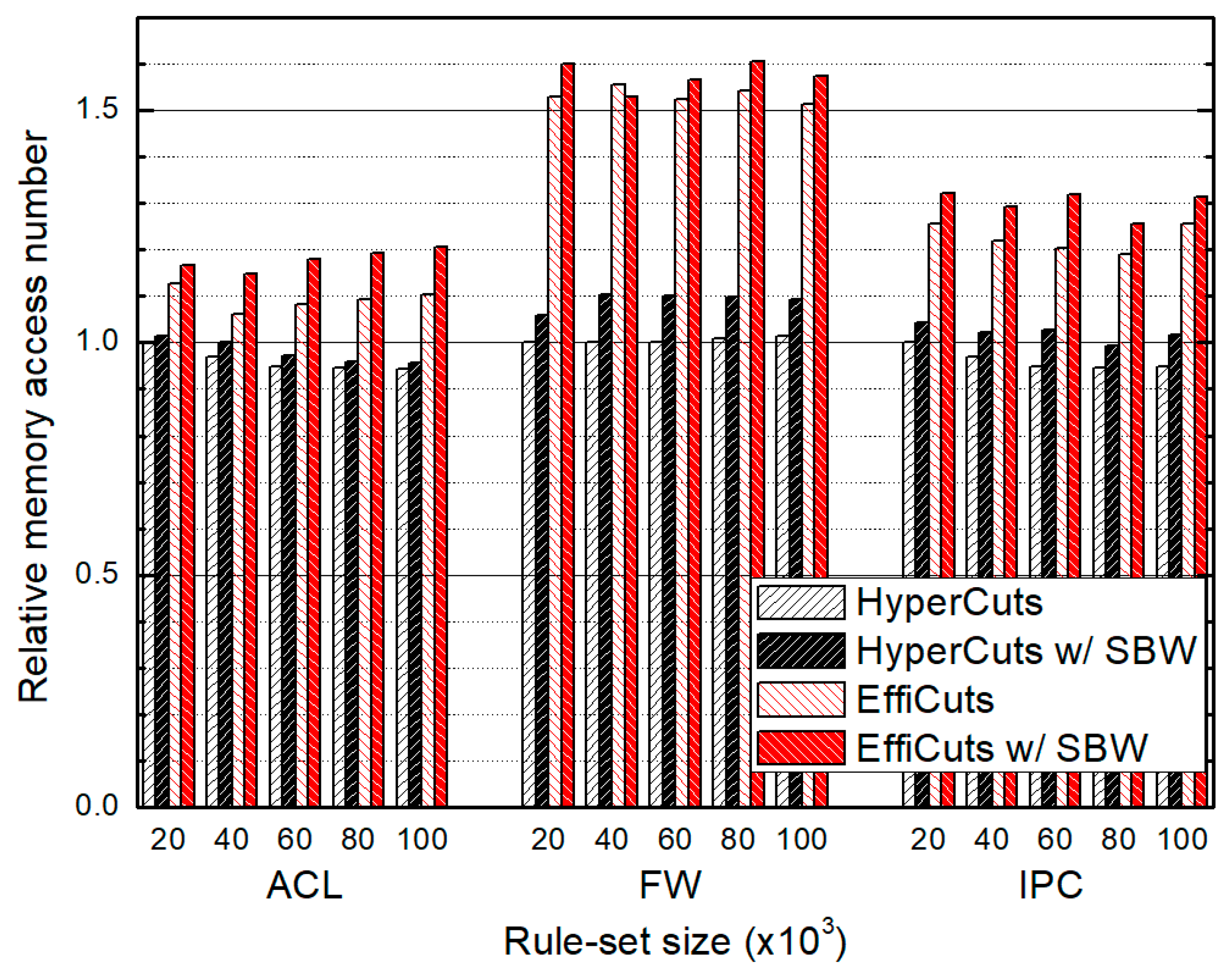
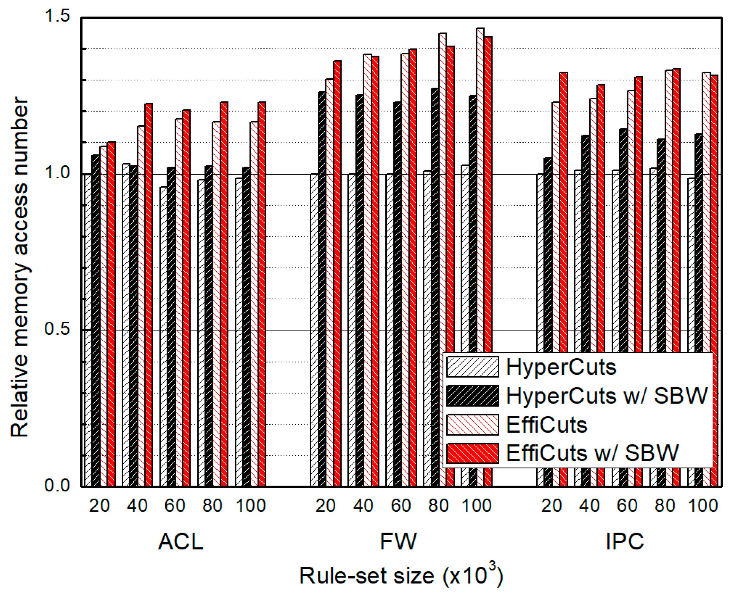
4.2. Packet Classification Performance
4.3. Table Building Time
5. Conclusions
Author Contributions
Funding
Conflicts of Interest
References
- Internet of Business. Available online: https://internetofbusiness.com/worldwide-connected-car-market-to-top-125-million-by-2022 (accessed on 9 April 2018).
- Asia Economy. Available online: http://www.asiae.co.kr/news/view.htm?idxno=2015060407474397851 (accessed on 9 June 2017).
- Gupta, P.; McKeown, N. Algorithms for Packet Classification. IEEE Netw. 2001, 15, 24–32. [Google Scholar] [CrossRef]
- Harada, T.; Tanaka, K.; Mikawa, K. Acceleration of Packet Classification via Inclusive Rules. In Proceedings of the 2018 IEEE Conference on Communications and Network Security (CNS), Beijing, China, 30 May–1 June 2018; pp. 1–2. [Google Scholar]
- Yahya, A.; Al-Nejadi, D.; Shaikh-Husin, N. Survey on Multi Field Packet Classification Techniques. Res. J. Recent Sci. 2015, 4, 98–106. [Google Scholar]
- Lim, H. Survey and Proposal on Packet Classification Algorithms. In Proceedings of the 2010 International Conference on High Performance Switching and Routing (HPSR), Richardson, TX, USA, 13–16 June 2010. [Google Scholar]
- Pagiamtzis, K.; Sheikholeslami, A. Content-Addressable Memory (CAM) Circuits and Architectures: A Tutorial and Survey. IEEE J. Solid-State Circuits 2006, 41, 712–727. [Google Scholar] [CrossRef]
- Pérez, K.G.; Yang, X.; Scott-Hayward, S.; Sezer, S. A Configurable Packet Classification Architecture for Software-Defined Networking. In Proceedings of the 2014 27th IEEE International System-on-Chip Conference (SOCC), Las Vegas, NV, USA, 2–5 September 2014. [Google Scholar]
- Pérez, K.G.; Yang, X.; Scott-Hayward, S.; Sezer, S. Optimized Packet Classification for Software-Defined Networking. In Proceedings of the 2014 IEEE International Conference on Communications (ICC), Sydney, NSW, Australia, 10–14 June 2014. [Google Scholar]
- Li, X.; Shao, Y. Memory compression for Recursive Flow Classification Algorithm in Network Packet Processing Devices. In Proceedings of the IEEE 3rd Advanced Information Technology, Electronic and Automation Control Conference (IAEAC), Chongqing, China, 12–14 October 2018; pp. 1502–1505. [Google Scholar]
- Yingchareonthawornchai, S.; Daly, J.; Liu, A.X.; Torng, E. A Sorted-Partitioning Approach to Fast and Scalable Dynamic Packet Classification. IEEE/ACM Trans. Netw. 2018, 26, 1907–1920. [Google Scholar] [CrossRef]
- Singh, S.; Baboescu, F.; Varghese, G.; Wang, J. Packet Classification Using Multidimensional Cutting. In Proceedings of the 2003 Conference on Applications, Technologies, Architectures, and Protocols for Computer Communications, New York, NY, USA, 25–29 August 2003. [Google Scholar]
- Wee, J.; Pak, W. Integrated Packet Classification to Support Multiple Security Policies for Robust and Low Delay V2X Services. Hindawi Mob. Inf. Syst. 2018, 7, 1–10. [Google Scholar] [CrossRef]
- Aloise, D.; Deshpande, A.; Hansen, P.; Popat, P. NP-hardness of Euclidean Sum-of-Squares Clustering. Mach. Learn. 2009, 75, 245–248. [Google Scholar] [CrossRef]
- Dasgupta, S.; Freund, Y. Random Projection Trees for Vector Quantization. IEEE Trans. Inf. Theory 2009, 55, 3229–3242. [Google Scholar] [CrossRef] [Green Version]
- Vamanan, B.; Voskuilen, G.; Vijaykumar, T.N. Efficuts: Optimizing packet classification for memory and throughput. In Proceedings of the 2010 ACM Special Interest Group Data Commun, New Delhi, India, 30 August–3 September 2010. [Google Scholar]
- Gupta, P.; McKeown, N. Classifying packets with hierarchical intelligent cuttings. IEEE Micro 2000, 20, 34–41. [Google Scholar] [CrossRef]
- Taylor, D.E.; Turner, J.S. ClassBench: A Packet Classification Benchmark. IEEE/ACM Trans. Netw. 2007, 15, 499–511. [Google Scholar] [CrossRef] [Green Version]


| Rule | Field 1 | Field 2 | Field 3 | Field 4 |
|---|---|---|---|---|
| Rule 1 | (0,8) | (0,1) | (0,2) | (0,5) |
| Rule 2 | (6,9) | (0,1) | (0,2) | (0,5) |
| Rule 3 | (0,15) | (4,5) | (4,5) | (0,5) |
| Rule 4 | (9,10) | (12,15) | (4,5) | (6,7) |
| Rule 5 | (6,15) | (6,10) | (4,5) | (6,7) |
| Rule 6 | (0,8) | (8,12) | (6,7) | (6,7) |
| Rule 7 | (0,2) | (13,15) | (6,7) | (6,7) |
| Field 1 | Field 2 | Field 3 | Field 4 | |
|---|---|---|---|---|
| Number of unique matching ranges | 6 | 6 | 3 | 2 |
| Average number of unique matching ranges | 4.5 | |||
| Number of wildcards | 4 | 0 | 0 | 0 |
| Average number of wildcards | 1.75 | |||
| 0.19 | 4.08 | 2.04 | 0.14 | |
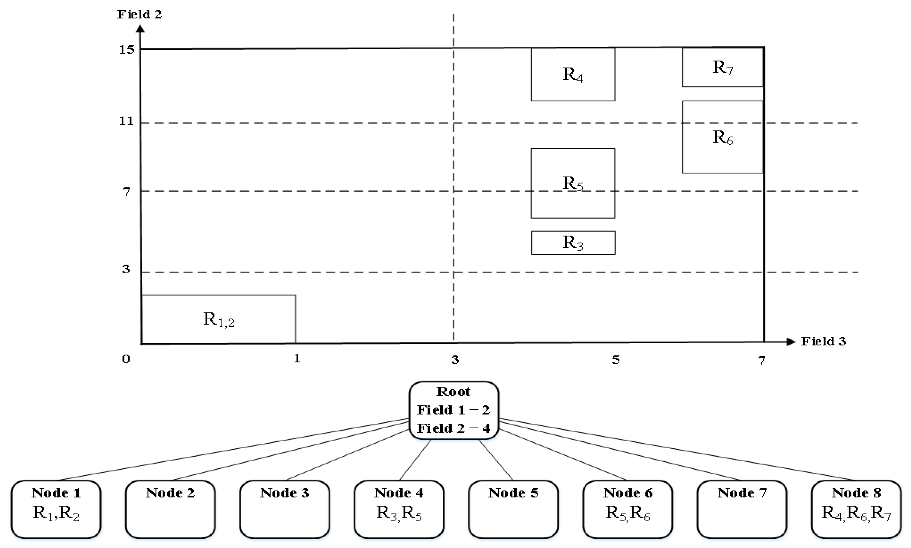
| Selected partitioning fields | Field 2, Field 3 | |||
© 2019 by the authors. Licensee MDPI, Basel, Switzerland. This article is an open access article distributed under the terms and conditions of the Creative Commons Attribution (CC BY) license (http://creativecommons.org/licenses/by/4.0/).
Share and Cite
Wee, J.; Choi, J.-G.; Pak, W. Wildcard Fields-Based Partitioning for Fast and Scalable Packet Classification in Vehicle-to-Everything. Sensors 2019, 19, 2563. https://doi.org/10.3390/s19112563
Wee J, Choi J-G, Pak W. Wildcard Fields-Based Partitioning for Fast and Scalable Packet Classification in Vehicle-to-Everything. Sensors. 2019; 19(11):2563. https://doi.org/10.3390/s19112563
Chicago/Turabian StyleWee, Jaehyung, Jin-Ghoo Choi, and Wooguil Pak. 2019. "Wildcard Fields-Based Partitioning for Fast and Scalable Packet Classification in Vehicle-to-Everything" Sensors 19, no. 11: 2563. https://doi.org/10.3390/s19112563
APA StyleWee, J., Choi, J.-G., & Pak, W. (2019). Wildcard Fields-Based Partitioning for Fast and Scalable Packet Classification in Vehicle-to-Everything. Sensors, 19(11), 2563. https://doi.org/10.3390/s19112563