A New Deep Learning Algorithm for SAR Scene Classification Based on Spatial Statistical Modeling and Features Re-Calibration


 ,
,  ,
, 
Abstract
1. Introduction
- (1)
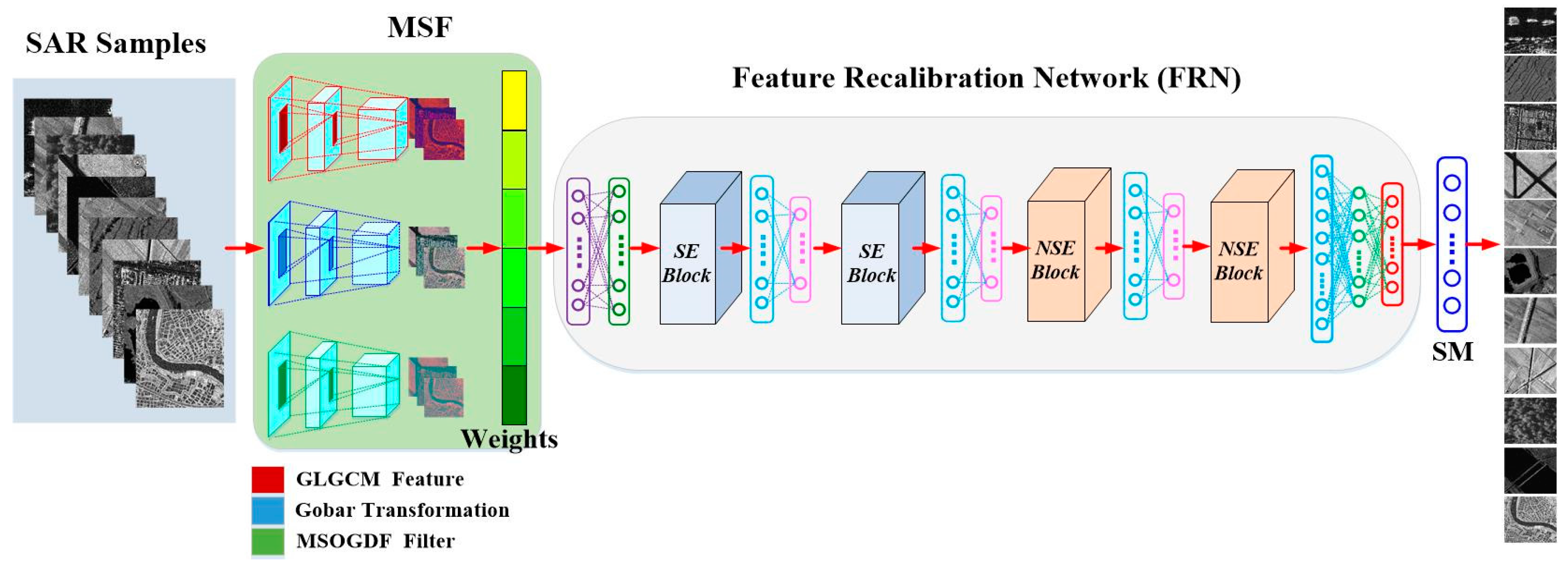
- A framework for SAR scene classification is proposed, which contains two parts: multi-scale spatial features (MSF) extraction and Features Recalibration Network (FRN). The first part aims to extract multi-scale low-level features, while the second part intends to extract high-level features and then confirm the types of targets.
- (2)
- An example of the MSF is presented, in which a Multi-Scale Omnidirectional Gaussian Derivative Filter (MSOGDF), a Gray Level Gradient Co-occurrence Matrix (GLGCM) and Gabor transformation are used to extract rich detailed information from SAR images.
- (3)
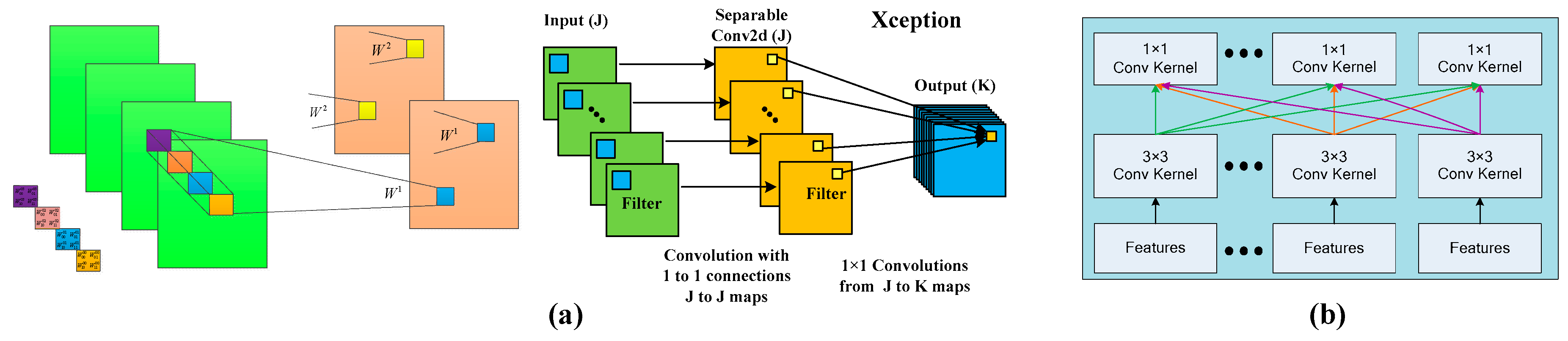
- An example of the FRN is demonstrated, in which Depthwise Separable Convolution (DSC), attention mechanism and CNN are integrated to better extract the high-level features of different types of targets.
- (4)
- A prototype of the above-mentioned framework is implemented and its performance is assessed using SAR data with different frequency bands and different resolutions.
2. Background
2.1. State of the Art
2.2. Deep Learning
3. Methodology
3.1. The Framework Architecture
3.2. Multi-Scale Spatial Feature (MSF)
3.2.1. GLGCM Extraction
- (1)
- Normalization processing for the image: . is the total number of gray levels, and is the maximum gray value of a given SAR image.
- (2)
- Computing the gray gradient image: .To better extract texture information, four Sobel operators in four directions with a 3 × 3 window are adopted considering the amount of calculation. They are 0°, 45°, 90° and 135°, which are denoted by , , , and respectively.Then, the gradient value of the pixel is computed by Equation (4):where the symbol means dot product operation between two matrices, and denotes 3 × 3 matrix values around the central pixel .
- (3)
- Gray gradient image normalization: . is the number of gray levels for the gray gradient image, and is the maximum value of the gradient matrix.
- (4)
- GLGCM computation: . It counts the number of the point pairs in the image which satisfies , simultaneously.
3.2.2. Gabor Transformation
3.2.3. Multi-Scale Omnidirectional Gaussian Derivative Filter (MSOGDF)
3.2.4. Multi-Scale Spatial Features (MSF) Fusion
3.3. Depthwise Separable Convolution (DSC)
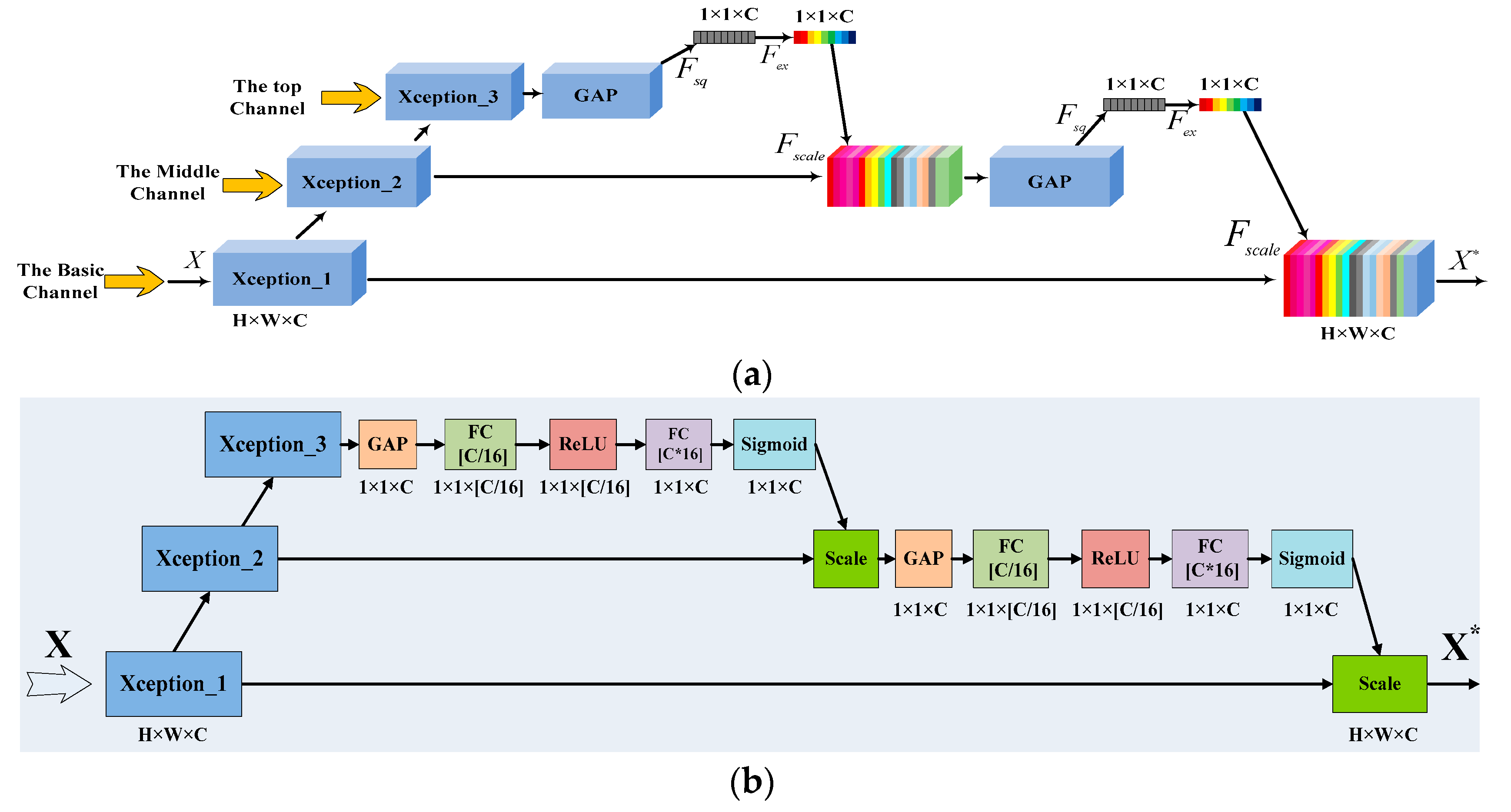
3.4. New Squeeze-And-Excitation (NSE) Block
4. Experiments and Results
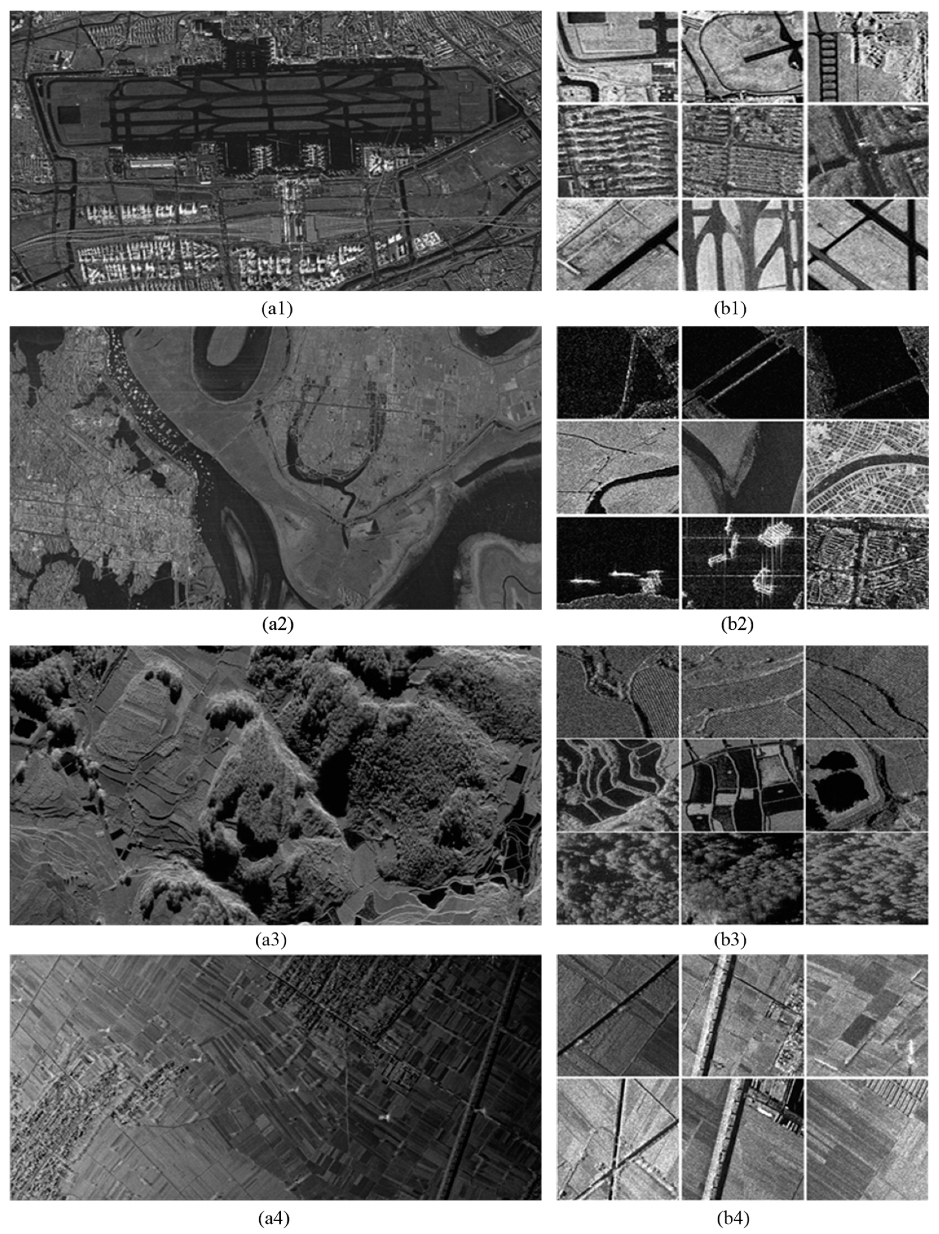
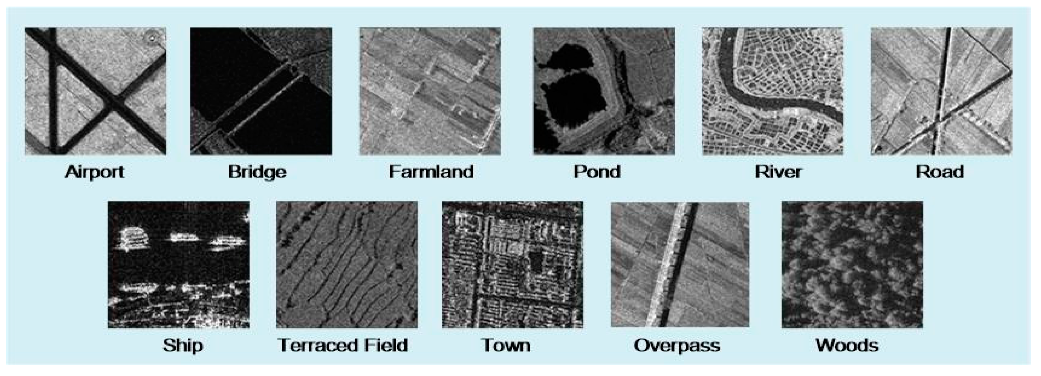
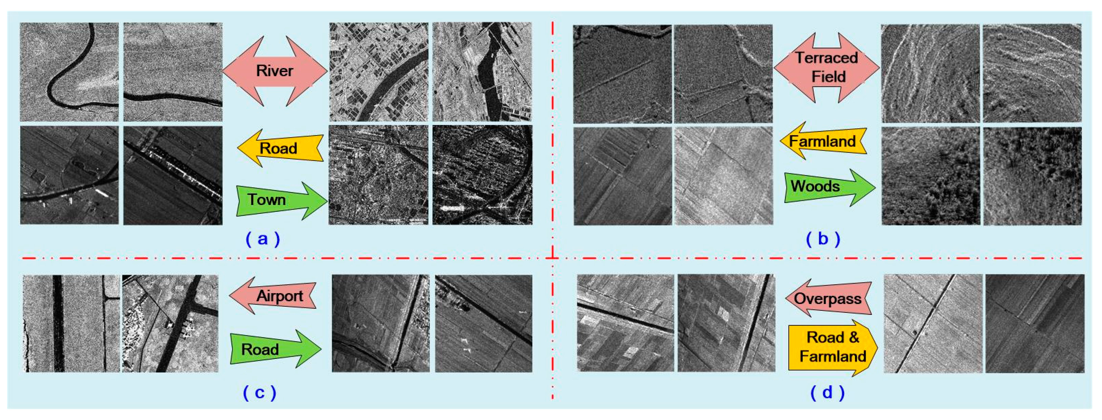
4.1. Datasets Used in this Study
4.2. Parameters Setting of the Proposed Framework
4.3. Results
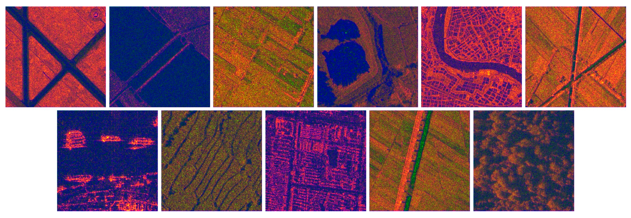
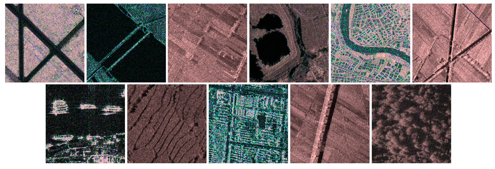
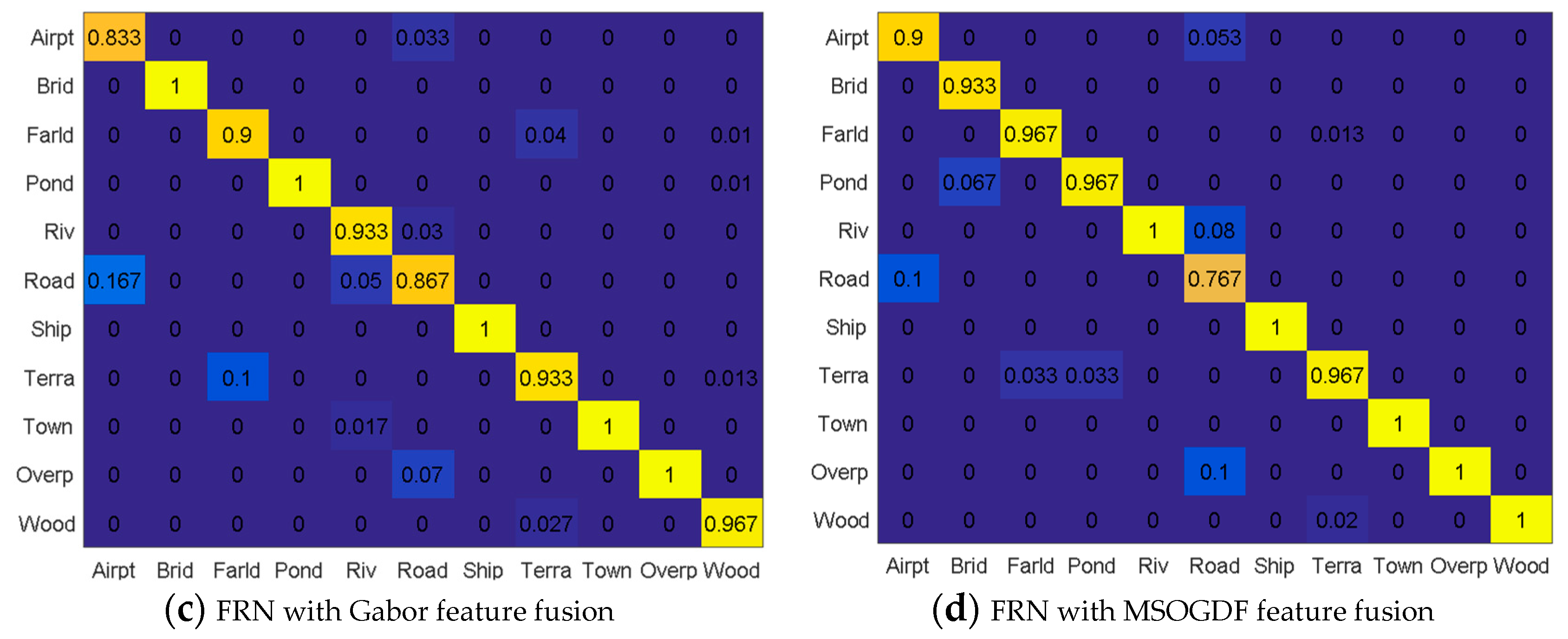
4.3.1. Multi-Scale Feature Extraction and Fusion
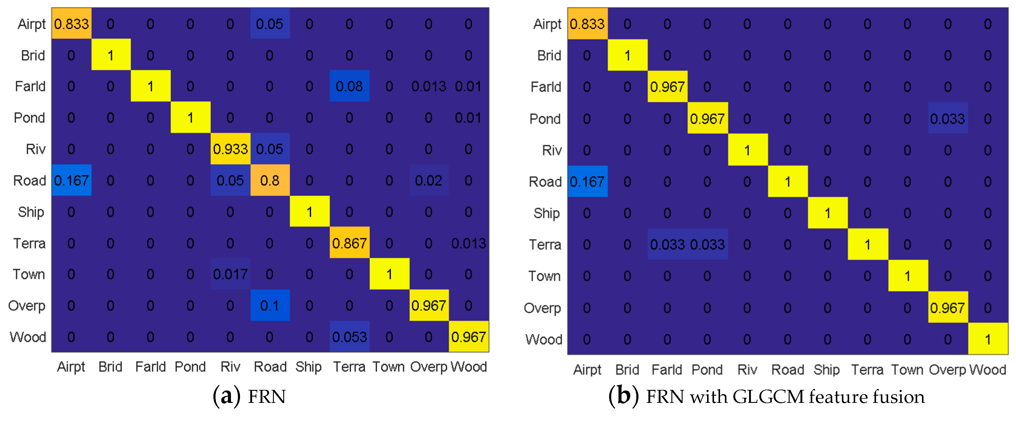
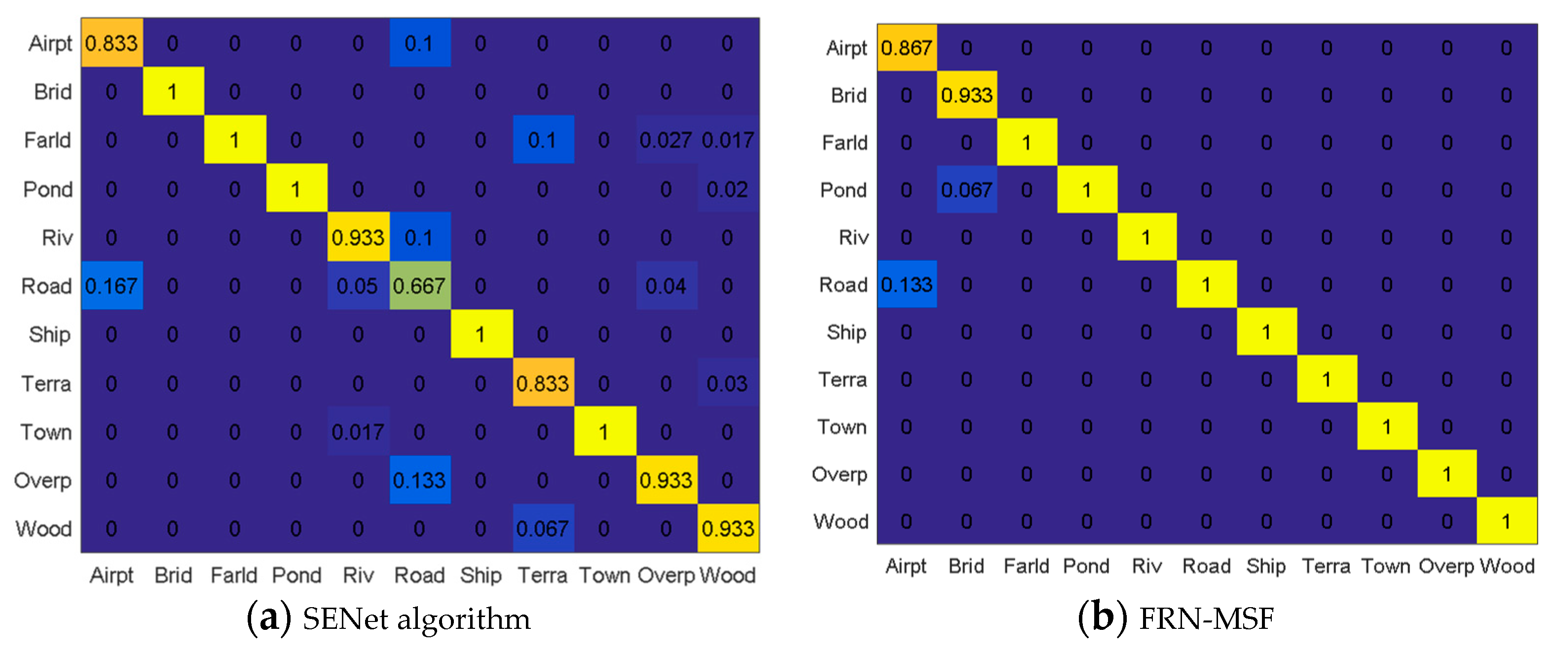
4.3.2. Performance Assessment
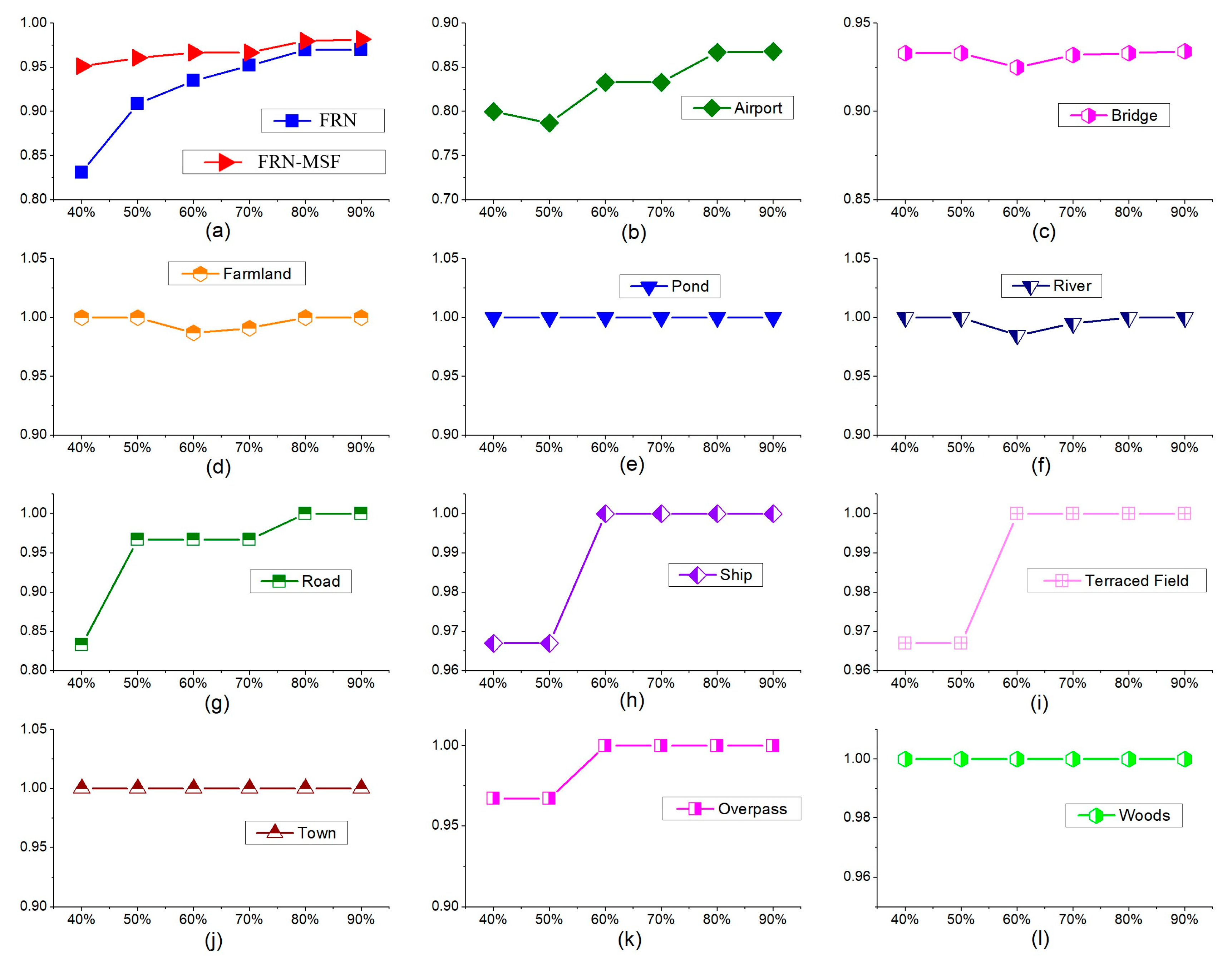
4.3.3. Impacts of the Training Sample Ratios on the Performance
4.3.4. Generalization
5. Discussion
6. Conclusions
Author Contributions
Funding
Acknowledgments
Conflicts of Interest
References
- Chen, J.; Wang, C.; Ma, Z.; Chen, J.; He, D.; Ackland, S. Remote sensing scene classification based on convolutional neural networks pre-trained using attention-guided sparse filters. Remote Sens. 2018, 10, 290. [Google Scholar] [CrossRef]
- Martha, T.R.; Kerle, N.; van Westen, C.J.; Jetten, V.; Kumar, K.V. Segment optimization and data-driven thresholding for knowledge-based landslide detection by object-based image analysis. IEEE Trans. Geosci. Remote Sens. 2011, 49, 4928–4943. [Google Scholar] [CrossRef]
- Lv, N.; Chen, C.; Qiu, T.; Sangaiah, A.K. Deep learning and superpixel feature extraction based on contractive autoencoder for change detection in SAR images. IEEE Trans. Ind. Inform. 2018, 14, 5530–5538. [Google Scholar] [CrossRef]
- Chen, H.; Jiao, L.; Liang, M.; Liu, F.; Yang, S.; Hou, B. Fast unsupervised deep fusion network for change detection of multitemporal SAR images. Neurocomputing 2019, 332, 56–70. [Google Scholar] [CrossRef]
- Li, Y.; Peng, C.; Chen, Y.; Jiao, L.; Zhou, L.; Shang, R. A Deep Learning Method for Change Detection in Synthetic Aperture Radar Images. IEEE Trans. Geosci. Remote Sens. 2019, 17, 8–16. [Google Scholar] [CrossRef]
- Zhu, Q.; Zhong, Y.; Zhao, B.; Xia, G.S.; Zhang, L. Bag-of-visual-words scene classifier with local and global features for high spatial resolution remote sensing imagery. IEEE Geosci. Remote Sens. Lett. 2016, 13, 747–751. [Google Scholar] [CrossRef]
- Lin, Z.; Ji, K.; Kang, M.; Leng, X.; Zou, H. Deep convolutional highway unit network for sar target classification with limited labeled training data. IEEE Geosci. Remote Sens. Lett. 2017, 14, 1091–1095. [Google Scholar] [CrossRef]
- Kang, M.; Ji, K.; Leng, X.; Xing, X.; Zou, H. Synthetic aperture radar target recognition with feature fusion based on a stacked autoencoder. Sensors 2017, 17, 192. [Google Scholar] [CrossRef] [PubMed]
- Kang, M.; Ji, K.; Leng, X.; Lin, Z. Contextual region-based convolutional neural network with multilayer fusion for SAR ship detection. Remote Sens. 2017, 9, 860. [Google Scholar] [CrossRef]
- Lin, Z.; Ji, K.; Leng, X.; Kuang, G. Squeeze and Excitation Rank Faster R-CNN for Ship Detection in SAR Images. IEEE Geosci. Remote Sens. Lett. 2018, 16, 751–755. [Google Scholar] [CrossRef]
- Zheng, X.; Sun, X.; Fu, K.; Wang, H. Automatic annotation of satellite images via multi-feature joint sparse coding with spatial relation constraint. IEEE Geosci. Remote Sens. Lett. 2013, 10, 652–656. [Google Scholar] [CrossRef]
- Wang, Y.; Zhang, L.; Tong, X.; Zhang, L.; Zhang, Z.; Liu, H.; Xing, X.; Mathiopoulos, P.T. A three-layered graph-based learning approach for remote sensing image retrieval. IEEE Trans. Geosci. Remote Sens. 2016, 54, 6020–6034. [Google Scholar] [CrossRef]
- Mishra, N.B.; Crews, K.A. Mapping vegetation morphology types in a dry savanna ecosystem: Integrating hierarchical object-based image analysis with Random Forest. Int. J. Remote Sens. 2014, 35, 1175–1198. [Google Scholar] [CrossRef]
- Phinn, S.R.; Roelfsema, C.M.; Mumby, P.J. Multi-scale, object-based image analysis for mapping geomorphic and ecological zones on coral reefs. Int. J. Remote Sens. 2012, 33, 3768–3797. [Google Scholar] [CrossRef]
- Meenakshi, A.V.; Punitham, V. Performance of speckle noise reduction filters on active radar and SAR images. Gop. Int. J. Technol. Eng. Syst. 2011, 1, 112–114. [Google Scholar]
- Cheng, G.; Han, J.; Lu, X. Remote sensing image scene classification: Benchmark and state of the art. Proc. IEEE 2017, 105, 1865–1883. [Google Scholar] [CrossRef]
- Ojala, T.; Pietikäinen, M.; Mäenpää, T. Multiresolution gray-scale and rotation invariant texture classification with local binary patterns. IEEE Trans. Pattern Anal. Mach. Intell. 2002, 7, 971–987. [Google Scholar] [CrossRef]
- Li, Y.; Tao, C.; Tan, Y.; Shang, K.; Tian, J. Unsupervised multilayer feature learning for satellite image scene classification. IEEE Geosci. Remote Sens. Lett. 2016, 13, 157–161. [Google Scholar] [CrossRef]
- Romero, A.; Gatta, C.; Camps-Valls, G. Unsupervised deep feature extraction for remote sensing image classification. IEEE Trans. Geosci. Remote Sens. 2016, 54, 1349–1362. [Google Scholar] [CrossRef]
- Zhang, F.; Du, B.; Zhang, L. Scene classification via a gradient boosting random convolutional network framework. IEEE Trans. Geosci. Remote Sens 2016, 54, 1793–1802. [Google Scholar] [CrossRef]
- Zhao, B.; Zhong, Y.; Zhang, L. A spectral–structural bag-of-features scene classifier for very high spatial resolution remote sensing imagery. ISPRS J. Photogramm. Remote Sens. 2016, 116, 73–85. [Google Scholar] [CrossRef]
- Hinton, G.E.; Salakhutdinov, R.R. Reducing the dimensionality of data with neural networks. Science 2006, 313, 504–507. [Google Scholar] [CrossRef]
- Hinton, G.E.; Osindero, S.; Teh, Y.W. A fast learning algorithm for deep belief nets. Neural Comput. 2006, 18, 1527–1554. [Google Scholar] [CrossRef]
- Krizhevsky, A.; Sutskever, I.; Hinton, G.E. Imagenet classification with deep convolutional neural networks. In Proceedings of the Advances in Neural Information Processing Systems, Lake Tahoe, NV, USA, 3–6 December 2012; pp. 1097–1105. [Google Scholar]
- Silver, D.; Huang, A.; Maddison, C.J.; Guez, A.; Sifre, L.; Van Den Driessche, G.; Dieleman, S. Mastering the game of Go with deep neural networks and tree search. Nature 2016, 529, 484. [Google Scholar] [CrossRef]
- Hartling, S.; Sagan, V.; Sidike, P.; Maimaitijiang, M.; Carron, J. Urban Tree Species Classification Using a WorldView-2/3 and LiDAR Data Fusion Approach and Deep Learning. Sensors 2019, 19, 1284. [Google Scholar] [CrossRef]
- Yang, J.; Jiang, Y.G.; Hauptmann, A.G.; Ngo, C.W. Evaluating bag-of-visual-words representations in scene classification. In Proceedings of the International Workshop on Workshop on Multimedia Information Retrieval, Augsburg, Germany, 24–29 September 2007; pp. 197–206. [Google Scholar]
- Hofmann, T. Unsupervised learning by probabilistic latent semantic analysis. Mach. Learn. 2001, 42, 177–196. [Google Scholar] [CrossRef]
- Cunningham, P.; Delany, S.J. k-Nearest neighbor classifiers. Mult. Classif. Syst. 2007, 34, 1–17. [Google Scholar]
- Cloude, S.R.; Pottier, E. An entropy-based classification scheme for land applications of polarimetric SAR. IEEE Trans. Geosci. Remote Sens. 1997, 35, 68–78. [Google Scholar] [CrossRef]
- Sheng, G.; Yang, W.; Xu, T.; Sun, H. High-resolution satellite scene classification using a sparse coding based multiple feature combination. Int. J. Remote Sens. 2012, 33, 2395–2412. [Google Scholar] [CrossRef]
- Cheng, G.; Guo, L.; Zhao, T.; Han, J.; Li, H.; Fang, J. Automatic landslide detection from remote-sensing imagery using a scene classification method based on BoVW and pLSA. Int. J. Remote Sens. 2013, 34, 45–59. [Google Scholar] [CrossRef]
- Hu, F.; Xia, G.S.; Wang, Z.; Huang, X.; Zhang, L.; Sun, H. Unsupervised feature learning via spectral clustering of multidimensional patches for remotely sensed scene classification. IEEE J. Sel. Top. Appl. Earth Obs. Remote Sens. 2015, 8, 2015–2030. [Google Scholar] [CrossRef]
- Aksoy, S.; Koperski, K.; Tusk, C.; Marchisio, G.; Tilton, J.C. Learning Bayesian classifiers for scene classification with a visual grammar. IEEE Trans. Geosci. Remote Sens. 2005, 43, 581–589. [Google Scholar] [CrossRef]
- Zhong, C.; Mu, X.; He, X.; Zhan, B.; Niu, B. Classification for SAR Scene Matching Areas Based on Convolutional Neural Networks. IEEE Geosci. Remote Sens. Lett. 2018, 15, 1377–1381. [Google Scholar] [CrossRef]
- Hu, J.; Shen, L.; Sun, G. Squeeze-and-excitation networks. In Proceedings of the IEEE Conference on Computer Vision and Pattern Recognition, IEEE, Salt Lake City, UT, USA, 18–22 June 2018; pp. 7132–7141. [Google Scholar]
- LeCun, Y.; Bottou, L.; Bengio, Y.; Haffner, P. Gradient-based learning applied to document recognition. Proc. IEEE 1998, 86, 2278–2324. [Google Scholar] [CrossRef]
- Xu, S.H.; Mu, X.D.; Zhao, P.; Ma, J. Scene classification of remote sensing image based on multi-scale feature and deep neural network. Acta Geod. Cartogr. Sin. China 2016, 45, 834–840. [Google Scholar]
- Geng, J.; Wang, H.; Fan, J.; Ma, X. Deep supervised and contractive neural network for SAR image classification. IEEE Trans. Geosci. Remote Sens. 2017, 55, 2442–2459. [Google Scholar] [CrossRef]
- Wang, H.; Dong, F. Image features extraction of gas/liquid two-phase flow in horizontal pipeline by GLCM and GLGCM. In Proceedings of the 2009 9th International Conference on Electronic Measurement & Instruments, IEEE, Beijing, China, 16–19 August 2009. [Google Scholar]
- Hua, B.O.; Fu-Long, M.A.; Li-Cheng, J. Research on computation of GLCM of image texture. Acta Electron. Sin. 2006, 1, 155–158. [Google Scholar]
- Li, H.C.; Celik, T.; Longbotham, N.; Emery, W.J. Gabor feature based unsupervised change detection of multitemporal SAR images based on two-level clustering. IEEE Geosci. Remote Sens. Lett. 2015, 12, 2458–2462. [Google Scholar]
- Liu, C.; Wechsler, H. Gabor feature based classification using the enhanced fisher linear discriminant model for face recognition. IEEE Trans. Image Process. 2002, 11, 467–476. [Google Scholar]
- Liu, J.; Tang, Z.; Zhu, J.; Tan, Z. Statistical modelling of spatial structures-based image classification. Control Decis. 2015, 30, 1092–1098. [Google Scholar]
- Simonyan, K.; Zisserman, A. Very deep convolutional networks for large-scale image recognition. arXiv 2014, 1409, 1556. [Google Scholar]
- Chollet, F. Xception: Deep learning with depthwise separable convolutions. In Proceedings of the IEEE Conference on Computer Vision and Pattern Recognition, IEEE, Honolulu, HI, USA, 21–26 July 2017; pp. 1251–1258. [Google Scholar]
- Sun, Y.; Fisher, R. Object-based visual attention for computer vision. Artif. Intell. 2003, 146, 77–123. [Google Scholar] [CrossRef]
- Firat, O.; Cho, K.; Sankaran, B.; Vural, F.T.Y.; Bengio, Y. Multi-way. multilingual neural machine translation. Comput. Speech Lang. 2017, 45, 236–252. [Google Scholar] [CrossRef]
- Nam, H.; Ha, J.W.; Kim, J. Dual attention networks for multimodal reasoning and matching. In Proceedings of the IEEE Conference on Computer Vision and Pattern Recognition, IEEE, Honolulu, HI, USA, 21–26 July 2017; pp. 299–307. [Google Scholar]
- Chorowski, J.K.; Bahdanau, D.; Serdyuk, D.; Cho, K.; Bengio, Y. Attention-based models for speech recognition. In Proceedings of the Advances in Neural Information Processing Systems, Montreal, QC, Canada, 7–12 December 2015; pp. 577–585. [Google Scholar]
- Zheng, H.; Fu, J.; Mei, T.; Luo, J. Learning multi-attention convolutional neural network for fine-grained image recognition. In Proceedings of the IEEE International Conference on Computer Vision, IEEE, Venice, Italy, 22–29 October 2017; pp. 5209–5217. [Google Scholar]
- Luo, W.; Schwing, A.G.; Urtasun, R. Efficient deep learning for stereo matching. In Proceedings of the IEEE Conference on Computer Vision and Pattern Recognition, Las Vegas, NV, USA, 1–26 June 2016; pp. 5695–5703. [Google Scholar]
- He, K.; Zhang, X.; Ren, S.; Sun, J. Identity mappings in deep residual networks. In Proceedings of the European Conference on Computer Vision, Amsterdam, The Netherlands, 11–14 October 2016; pp. 630–645. [Google Scholar]
- Szegedy, C.; Ioffe, S.; Vanhoucke, V.; Alemi, A.A. Inception-v4, inception-resnet and the impact of residual connections on learning. In Proceedings of the Thirty-First AAAI Conference on Artificial Intelligence, San Francisco, CA, USA, 4–9 February 2017. [Google Scholar]
- Xie, S.; Girshick, R.; Dollár, P.; Tu, Z.; He, K. Aggregated residual transformations for deep neural networks. In Proceedings of the IEEE Conference on Computer Vision and Pattern Recognition, IEEE, Honolulu, HI, USA, 21–26 July 2017; pp. 1492–1500. [Google Scholar]
- Huang, G.; Liu, Z.; Van Der Maaten, L.; Weinberger, K.Q. Densely connected convolutional networks. In Proceedings of the IEEE Conference on Computer Vision and Pattern Recognition, IEEE, Honolulu, HI, USA, 21–26 July 2017; pp. 4700–4708. [Google Scholar]
- Han, D.; Kim, J.; Kim, J. Deep pyramidal residual networks. In Proceedings of the IEEE Conference on Computer Vision and Pattern Recognition, IEEE, Honolulu, HI, USA, 21–26 July 2017; pp. 5927–5935. [Google Scholar]


| System | Platform | Band | Resolution (m) | Size(pixels) | Location (China) |
|---|---|---|---|---|---|
| TerraSAR-X | Satellite | X | 3 | 14,804 × 30,623 | Dongtinghu, Foshan |
| Gaofen-3 | Satellite | C | 1 | 31,699 × 26,193 | Airports (i.e., Shanghai) |
| MM-InSAR | Airborne | Millimeter | 0.15 | 10,240 × 13,050 | Xi’an |
| CAS-InSAR | Airborne | X | 0.5 | 16,384 × 16,384 | Weinan |
| Layer Types | Convolutions/Pooling Window Size |
|---|---|
| Input | − |
| Conv2D Convolution Layer C1 | 5 × 5 × 96 |
| Pooling S1 | 2 × 2 |
| SE Block_1 | − |
| Conv2D Convolution Layer C2 | 3 × 3 × 256 |
| Pooling S2 | 2 × 2 |
| SE Block_2 | − |
| Conv2D Convolution Layer C3 | 3 × 3 × 256 |
| Pooling S3 | 2 × 2 |
| NSE Block_1 | − |
| Conv2D Convolution Layer C4 | 3 × 3 × 512 |
| Pooling S4 | 2 × 2 |
| NSE Block_2 | − |
| FC_1 | 1024 |
| FC_2 | 1024 |
| FC_3 | 11 |
| Softmax | − |
| Group | 45° Group | 90° Group | 135° Group |
|---|---|---|---|
| Average Accuracy | 95.45% | 94.24% | 94.55% |
| Gabor Transformation | GLGCM Feature | MSOGDF Filter | |
|---|---|---|---|
| Airport | 0 | 0 | 1 |
| Bridge | 1 | 1 | 0 |
| Farmland | 0 | 0 | 0 |
| Pond | 1 | 0 | 0 |
| River | 0 | 1 | 1 |
| Road | 0 | 1 | 0 |
| Ship | 0 | 0 | 0 |
| Terraced field | 0 | 1 | 0 |
| Town | 0 | 1 | 1 |
| Overpass | 1 | 0 | 1 |
| Woods | 0 | 1 | 1 |
| Algorothm | MA (%) |
|---|---|
| SENet | 92.11 |
| FRN | 94.24 |
| FRN-Gabor | 94.85 |
| FRN-GLGCM | 97.58 |
| FRN-MSOGDF | 95.46 |
| FRN-MSF | 98.18 |
| Training Sample Ratio | 40% | 50% | 60% | 70% | 80% | 90% |
|---|---|---|---|---|---|---|
| Classification MA of FRN | 89.09 | 91.81 | 92.72 | 93.33 | 93.94 | 93.95 |
| Classification MA of FRN-MSF | 95.15 | 96.07 | 96.67 | 96.67 | 98.18 | 98.20 |
© 2019 by the authors. Licensee MDPI, Basel, Switzerland. This article is an open access article distributed under the terms and conditions of the Creative Commons Attribution (CC BY) license (http://creativecommons.org/licenses/by/4.0/).
Share and Cite
Chen, L.; Cui, X.; Li, Z.; Yuan, Z.; Xing, J.; Xing, X.; Jia, Z. A New Deep Learning Algorithm for SAR Scene Classification Based on Spatial Statistical Modeling and Features Re-Calibration. Sensors 2019, 19, 2479. https://doi.org/10.3390/s19112479
Chen L, Cui X, Li Z, Yuan Z, Xing J, Xing X, Jia Z. A New Deep Learning Algorithm for SAR Scene Classification Based on Spatial Statistical Modeling and Features Re-Calibration. Sensors. 2019; 19(11):2479. https://doi.org/10.3390/s19112479
Chicago/Turabian StyleChen, Lifu, Xianliang Cui, Zhenhong Li, Zhihui Yuan, Jin Xing, Xuemin Xing, and Zhiwei Jia. 2019. "A New Deep Learning Algorithm for SAR Scene Classification Based on Spatial Statistical Modeling and Features Re-Calibration" Sensors 19, no. 11: 2479. https://doi.org/10.3390/s19112479
APA StyleChen, L., Cui, X., Li, Z., Yuan, Z., Xing, J., Xing, X., & Jia, Z. (2019). A New Deep Learning Algorithm for SAR Scene Classification Based on Spatial Statistical Modeling and Features Re-Calibration. Sensors, 19(11), 2479. https://doi.org/10.3390/s19112479