1. Introduction
As typical wideband signals with rapidly time-varying frequency and large time-bandwidth product, linear frequency modulated (LFM) signals have been widely adopted in radar [
1], sonar [
2], mobile communications [
3], and seismic detection fields. Direction of arrival (DOA) estimation for wideband LFM signals has played an important role in position [
4], navigation and interference suppression [
5] of these fields.
Due to the wideband nonstationary characteristics of the LFM signals, the traditional high-resolution DOA estimation methods based on narrowband and wide-sense stationary signals [
6,
7,
8] cannot be applied for wideband LFM signals. The typical wideband DOA estimation methods include the incoherent signal-subspace method (ISM) [
9] and the coherent signal-subspace method (CSM) [
10]. The ISM decomposes the wideband signals into several independent narrowband signals by using discrete Fourier transform (DFT), and approximately assumes that the frequency is time-invariant in every frequency bin without taking the whole wideband information into account. Thus, it has a large amount of calculation and is invalid for the coherent signals. The CSM transforms the wideband signal into a certain reference frequency by the focusing matrices and takes the average of the covariance matrix to decorrelation. Although the CSM improves the accuracy of the wideband DOA estimation and has relatively low computational complexity, the focusing matrices are sensitive to a priori knowledge of the DOA which is hard to be known beforehand.
With the development of the time-frequency (TF) analysis methods, the special concentration property of wideband nonstationary signals in the TF domain can be used to distinguish from stationary signals and estimate its time-frequency signature, which motivates several approaches for the DOA estimation of wideband nonstationary signals. In [
11], the DOA estimation for wideband LFM signals is realized by interpolating the spatial time–frequency distribution (STFD) matrices. Besides the disturbance of cross-terms induced by the choice of the time–frequency points, this approach mainly suffers from time consuming and model biases. To improve the performance of wideband DOA estimation, several modified algorithms based on the short-time Fourier transform (STFT) [
12] and Wigner–Ville distribution (WVD) [
13] have been presented. Nevertheless, the narrow time-window in STFT limits the time–frequency resolution, and the WVD requires great computational cost and suffers from cross-terms interference when nonstationary signals are multicomponent. As a linear transformation without the cross-terms interference, the fractional Fourier transform (FRFT) has no frequency point selection problem in secondary TF distribution, and can be considered as a rotation operator in the TF plane [
14,
15]. Moreover, owing to the excellent aggregation characteristic for the LFM signals, the FRFT is especially suitable to deal with wideband LFM signals compared with other TF analysis approaches. By using the FRFT and multiple signal classification (FRFT-MUSIC) algorithm, the DOA estimation of uncorrelated wideband LFM signals based on uniform linear array (ULA) is presented in [
16], and the new received model in the fractional Fourier (FRF) domain is constructed, but it is invalid for coherent signals. The DOA estimations of coherent wideband LFM signals are proposed in [
17,
18] by performing a subspace smoothing and Toeplitz decorrelation scheme on the covariance matrix in FRF domain, respectively, at the cost of a reduction in array aperture.
Meanwhile, compressive sensing (CS) and sparse representation (SR) have been rapidly developed, and the spatial sparsity has been introduced in the DOA estimation of wideband signals. In [
19,
20], using the idea of the ISM or the CSM methods, the wideband signals are decomposed or transformed into narrowband signals, and then the spatial sparse solution of DOA is obtained by using the CS algorithms, such as orthogonal matching pursuit (OMP) [
19] or singular value decomposition (
-SVD) reconstruction [
20]. Motivated by the FRFT-MUSIC algorithm, the received model of wideband signals in the FRF domain is in accordance with the CS framework, and the spatial sparse solution of DOA can be recovered under the maximizing a posteriori (MAP) criterion based on
norm [
21]. In [
22], a spatial compressed sensing framework is employed for DOA estimation with a randomly thinned phased array. The above methods based on the CS framework are also applicable to correlated sources, even with a single snapshot. However, there is an inherent disadvantage in these methods, i.e., the grid mismatch problem, which is inevitable to bring substantial bias especially when the DOAs of signals deviate from the discrete grids or SNR increases. Their performance would be compromised with the grid sparsity in the CS methods. Furthermore, the aforementioned CS-based and TF-based algorithms are all based on ULA or random array, so the degrees of freedom (DOFs) are limited by the number of physical sensors, i.e., the number of wideband signals identified by these methods should be less than the number of physical sensors in the array.
In order to increase DOFs and address the scenario where the number of signal sources is more than that of physical sensors, the nested arrays [
23] and the coprime arrays [
24,
25,
26,
27,
28,
29], as two typical sparse arrays, have been used in the underdetermined DOA estimation algorithms. In [
24,
25,
26,
27,
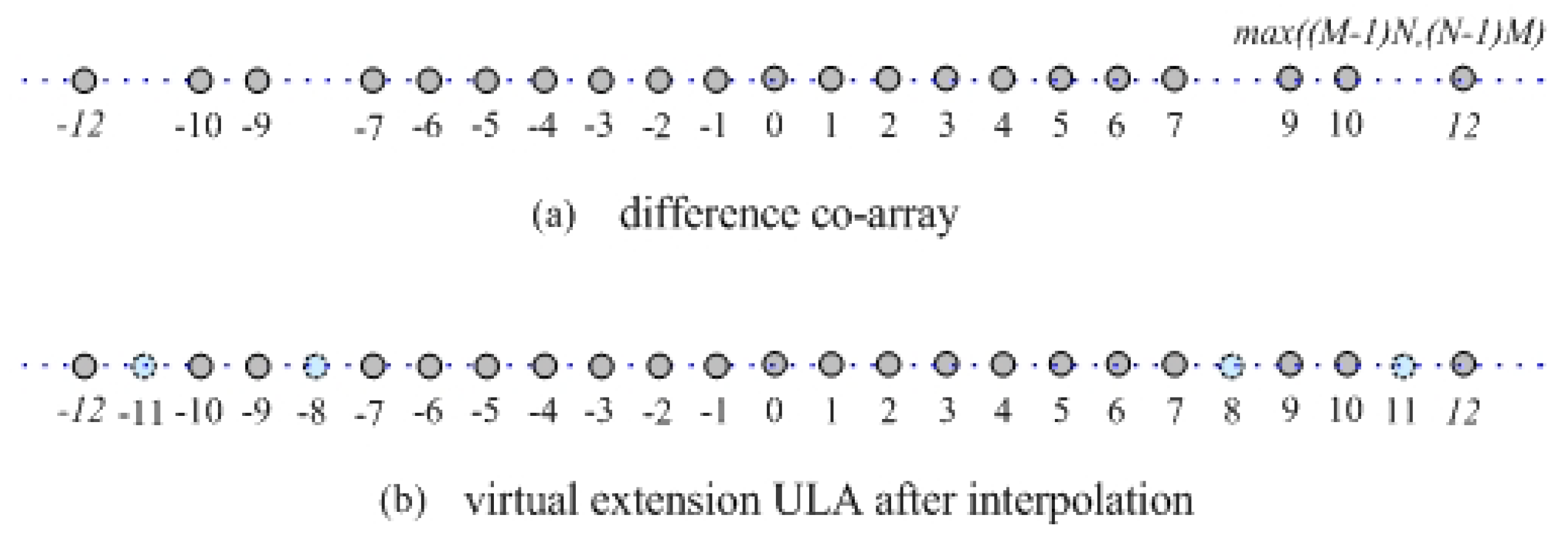
28], by adopting a coprime array as the received array of narrowband signals, a virtual extended array is constructed by vectoring the covariance matrix, which is also called the difference co-array. Although the difference co-array has some holes, which make it discontiguous, there are more virtual sensors in it than the physical sensors in a coprime array. In [
26,
27], discrete grids are defined at the spatial directions and the CS framework is used in the difference co-array, so the underdetermined DOA estimation of a narrowband signal is transformed to a spatial sparse recovery problem based on the CS framework, and many CS recovery algorithms, such as the least absolute shrinkage and selection operator (LASSO) [
26] and the OMP [
27], can be adopted. Nevertheless, the grid mismatch problem still exists due to the usage of the CS algorithms. In [
29], by extending the difference co-array to wideband cases, a two-step off-grid group sparsity approach for wideband DOA estimation is proposed to solve the underdetermined and grid mismatch problem. It firstly yields a coarser grid estimation, and then a bias vector is estimated by the optimization. However, it still uses the idea of ISM with time-invariant frequency and steering vector in every frequency bin, and mismatches with the wideband LFM signals model, which has the contiguous and linearly time-varying frequency and the time-variant steering vector. Moreover, the off-grid DOA estimation is still based on the discrete grids of spatial parameters, so the recovery deviation is only improved to a certain extent.
Recently, the grid-free compressed sensing approach based on a continuous dictionary has been proposed by atomic norm minimization (ANM) [
30], which can recover continuous-valued frequencies of the spectrally sparse signal from a few time-domain samples. Authors of [
31] modified the ANM to recover super-resolution frequencies with the prior knowledge from the structure of a spectrally sparse and undersampled signal. In [
32], an iterative reweighted ANM algorithm is proposed to improve frequency recovery performance with faster speed. Although these methods are applied to recover continuous-valued frequencies in spectral estimation, they provide an effective approach to solve the discrete grid mismatch problem for non-uniformly sampled or irregularly spaced signals.
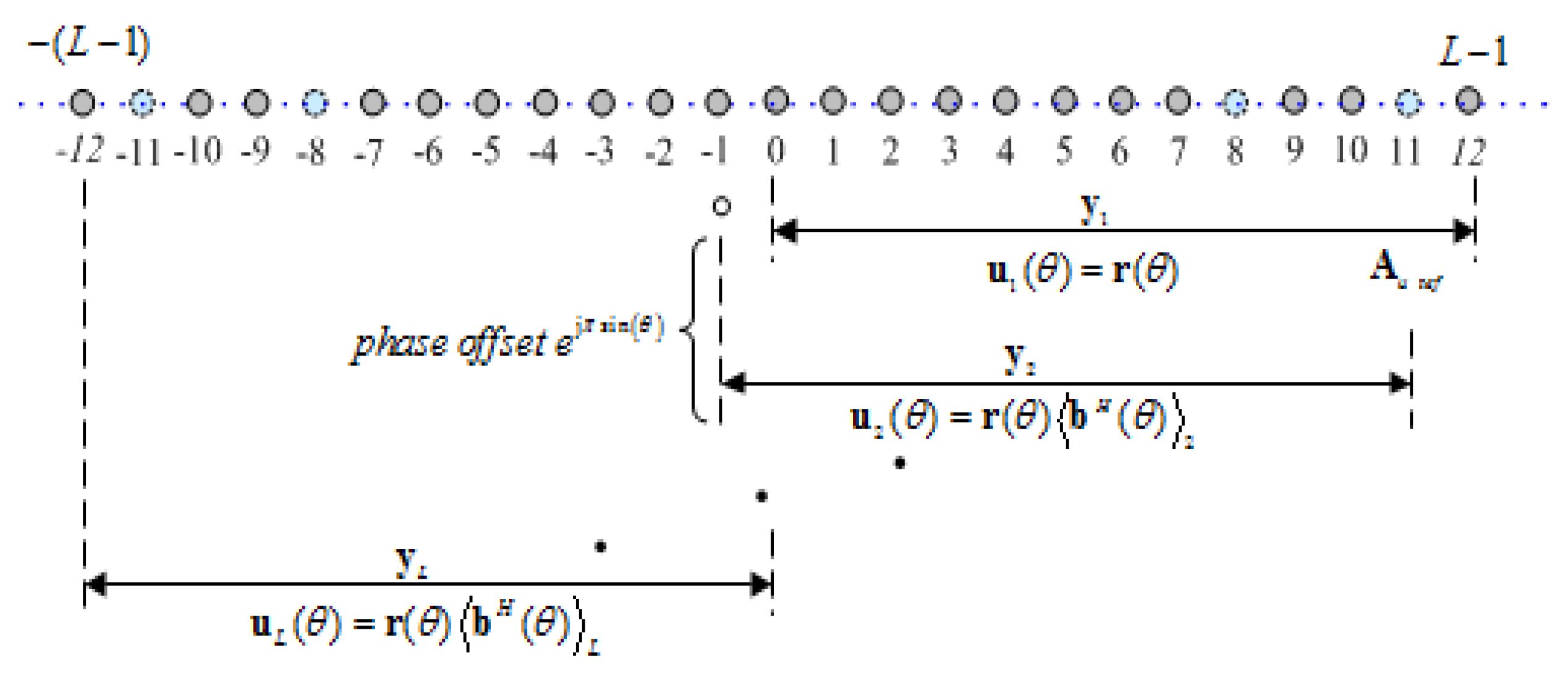
The focus of the proposed method is to solve the underdetermined DOA estimation of wideband LFM signals with gridless sparse reconstruction. By using the concentration property of wideband LFM signals in the FRF domain, the received sparse model in the FRF domain is firstly constructed based on the coprime array. Then, by interpolating virtual sensors into a difference co-array, the sparse covariance matrix of virtual ULA is recovered by modified atomic norm minimization, which increases the DOFs and provides a contiguous basis to avoid discrete grids mismatch. Unlike some existing algorithms that assume the steering vector of wideband signals is time-invariant in every frequency bin, the proposed method not only can resolve more wideband LFM sources than physical sensors with time-variant steering vector in FRF domain, but can also obtain more accurate DOA estimation performance with gridless sparse reconstruction.
Notations: The superscripts , , and respectively represent the transpose, conjugation, conjugate transpose and inverse of a matrix. Let the operator rank and Tr indicate the rank and the trace of a matrix, respectively. The notation ⊗ and ⊙ respectively signify the Kronecker product and Hadamard product between matrices. and mean the Frobenius norm and cardinality of a set, respectively.
4. Simulation Results
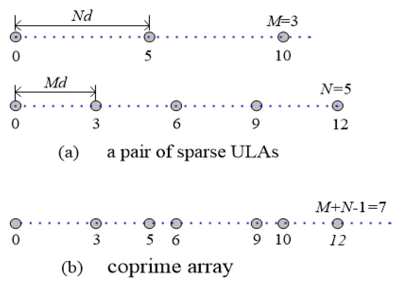
In this section, the simulation results will be presented to verify the performance of the proposed method with respect to resolution, DOFs and accuracy of DOA estimation. Consider a pair of coprime arrays with
isotropic physical sensors located at
, where
M = 3 and
N = 5. As for the wideband LFM signals, the ratio between bandwidth and the center frequency
is equal to 2/3. The sampling frequency
is three times as much as the highest frequency of the signal. The number of snapshots is P = 1024. For simplicity, assume that the power of wideband LFM signal is
, the SNR is defined as
. The proposed method would be compared with the wideband DOA estimation algorithms based on incoherent signal-subspace method (ISM) [
9], FRFT (FRFT-MUSIC) [
16], sparse representation with
-norm (FRFT-MAP) [
21], sparse sampling MUSIC (FRFT-CSSM) [
25], sparse recovery by compressive sensing (FRFT-OMP) [
27] nuclear norm sparse recovery (FRFT-NN) [
28] and spatial compressive sensing using randomly thinned array (ISM-CSRTA) [
22], respectively. FRFT-CSSM, FRFT-OMP and FRFT-NN methods are obtained by performing FRFT on the received signals and then using CSSM, OMP and nuclear norm algorithms to estimate DOAs, respectively. The interval of the pre-defined grids is set to
for the FRFT-MAP, FRFT-OMP and ISM-CSRTA algorithms. The penalty factor
for the proposed algorithm is set to be 0.25.
The first simulation takes the resolution of DOA estimation into consideration, and assumes that there are two closely spaced wideband LFM signals impinging on the coprime array with SNR = 10 dB, respectively. The first wideband signal comes from
=
fixedly, and the DOA of the second wideband signal is set as
=
+
, where
is the angular difference varied from
to
. That is also to say the second LFM signal comes from
and
, respectively. In
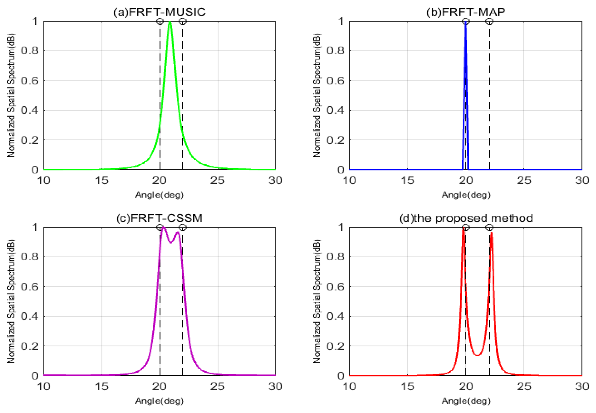
Figure 5, when
is
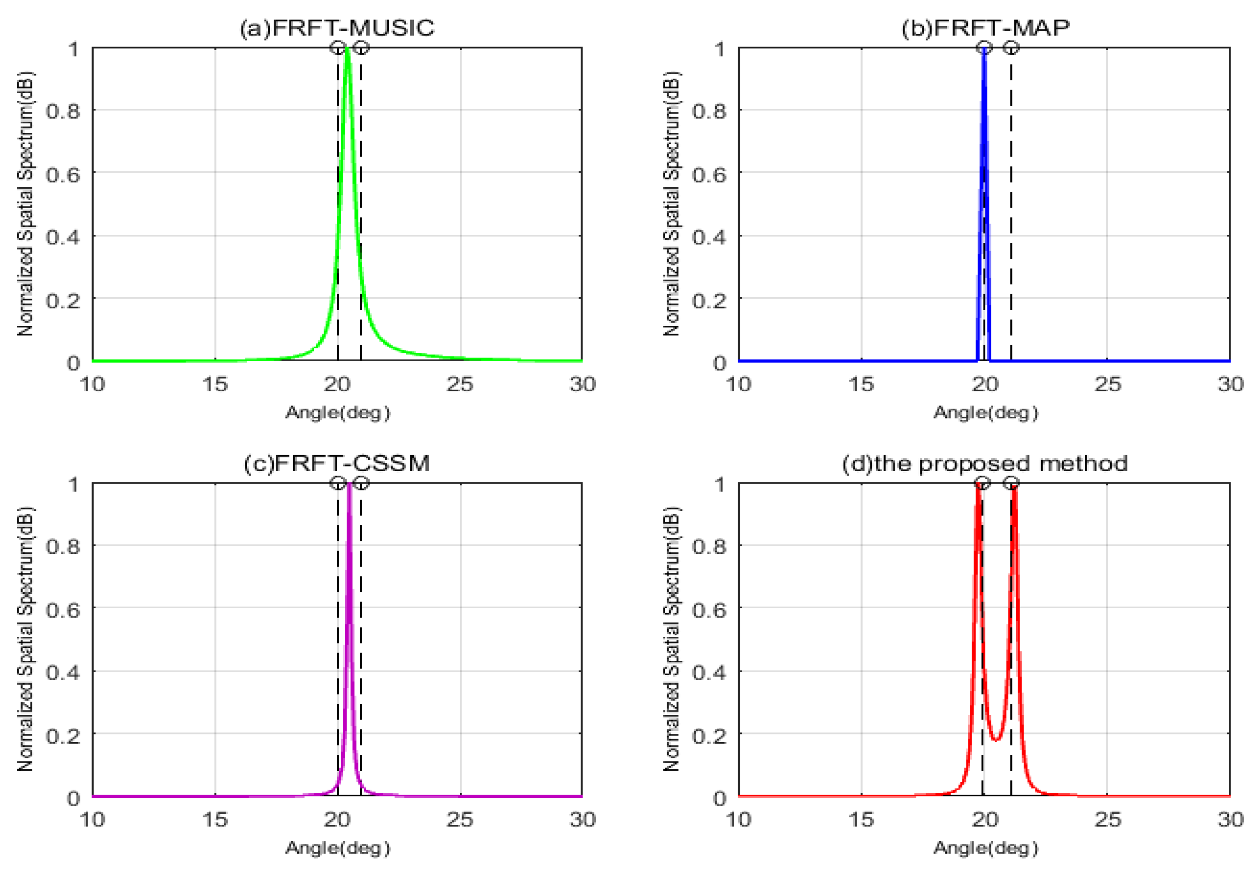
, it can be clearly seen that the FRFT-MUSIC and FRFT-MAP are unable to resolve the two signals, but FRFT-CSSM and the proposed method can accurately estimate DOAs of two wideband signals. That is because FRFT-MUSIC and FRFT-MAP methods are both based on ULA, which results in their resolutions constricted by the number of physical sensors in ULA. If the DOAs of two wideband signals stay too close, which exceeds their resolution abilities, these two methods cannot distinguish the DOAs of signals. FRFT-CSSM and the proposed method are based on the coprime array, and their DOFs are extended by vectoring covariance matrix, which are greater than the number of physical sensors, so their resolutions have been improved. Meanwhile, compared FRFT-CSSM with the proposed method in
Figure 5c,d, we can observe that although peaks of FRFT-CSSM point at the directions of wideband signals, its spectrum is not as sharp as that of the proposed method. Theoretically speaking, this is because the FRFT-CSSM algorithm only exploits the consecutive part in the difference co-array and discards the information of the non-consecutive part, its DOF is smaller than that of the proposed method and its resolution would decline. As shown in
Figure 6, when
decreases to
, the FRFT-MUSIC, FRFT-MAP and FRFT-CSSM methods all fail to identify the two sources, but only the proposed method has two shape peaks at the DOAs of two closely spaced signals. This is because the proposed method not only uses all the sensors in the difference co-array, but also interpolates virtual sensors whose information is recovered by the gridless sparse reconstruction. It exhibits a more superior resolution than the other algorithms with the same number of physical sensors, owing to the DOF increase.
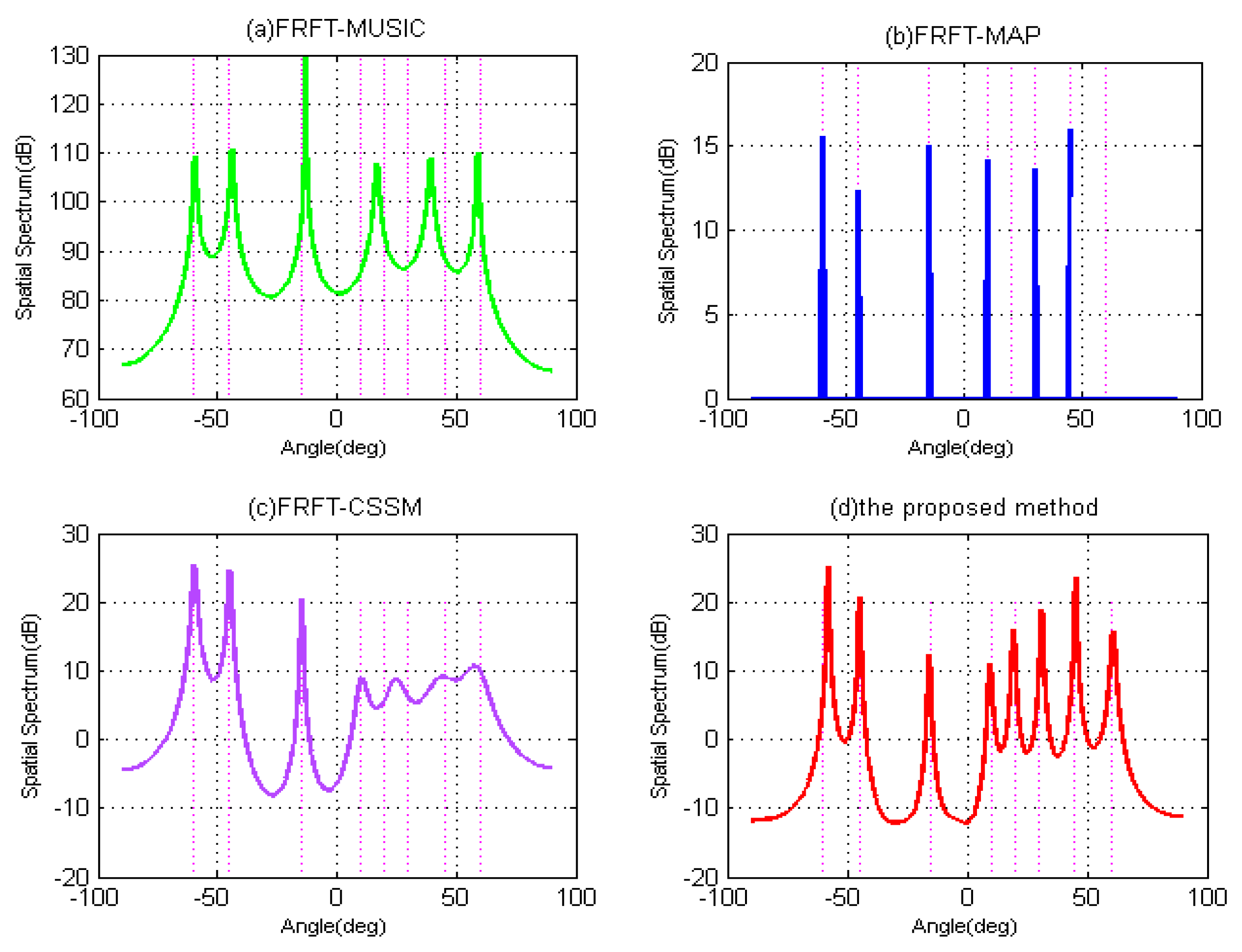
In what follows, to validate the DOFs improvement by the proposed method, the second simulation is carried out, when the number of wideband LFM signals exceeds the number of physical sensors. The tested algorithms all use seven physical sensors in received array with SNR = 10 dB and P = 1024. In
Figure 7, suppose that there are eight uncorrelated wideband signals arriving from different directions
impinging on the array, which are drew as the vertical pink lines in
Figure 7. As can be seen in
Figure 7a–c, while the number of signals surpasses the DOFs of algorithms, the FRFT-MUSIC, FRFT-MAP and FRFT-CSSM methods only can resolved some signals, but the other peaks of spatial spectrum become flatter and mix together, which results in the loss of DOAs of some signals and the unprecise resolution. Theoretically, FRFT-MUSIC and FRFT-MAP methods are both based on ULA, and their DOFs cannot be greater than the number of physical sensors, i.e., DOF ≤ 7, which are not able to estimate 8 uncorrelated signals simultaneously. As for FRFT-CSSM, because it is based on coprime array with seven sensors, the number of available consecutive virtual sensors in the difference co-array is increased to eight. Its DOF ≤ 8, which means it can resolve seven uncorrelated signals at most. In
Figure 7d, it can be clearly observed that when there are eight wideband signals impinging on the array, the proposed method has the ability to estimate their DOAs correctly at the same time. The number of available sensors is significantly increased to
by interpolating the virtual sensors. That is also to say the DOF of the proposed method reaches 13, and it can resolve 12 different wideband signals at most. Hence, when there are eight wideband signals impinging on the array, the other algorithms all fail, but the proposed method is valid to estimate the DOAs of eight or more wideband signals accurately.
Afterwards, the accuracy performance of DOA estimation algorithms would be assessed by the subsequent simulations in detail. The root mean square error (RMSE) of the DOA estimations is adopted as the performance index
where
is the estimation of
for the
qth Monte Carlo trial,
K is the number of wideband LFM signals and
Q denotes the number of Monte Carlo trials. In subsequent simulations, we run 500 Monte Carlo trials for each level. Consider the three signals impinging on the coprime array come from distinct directions
, respectively.
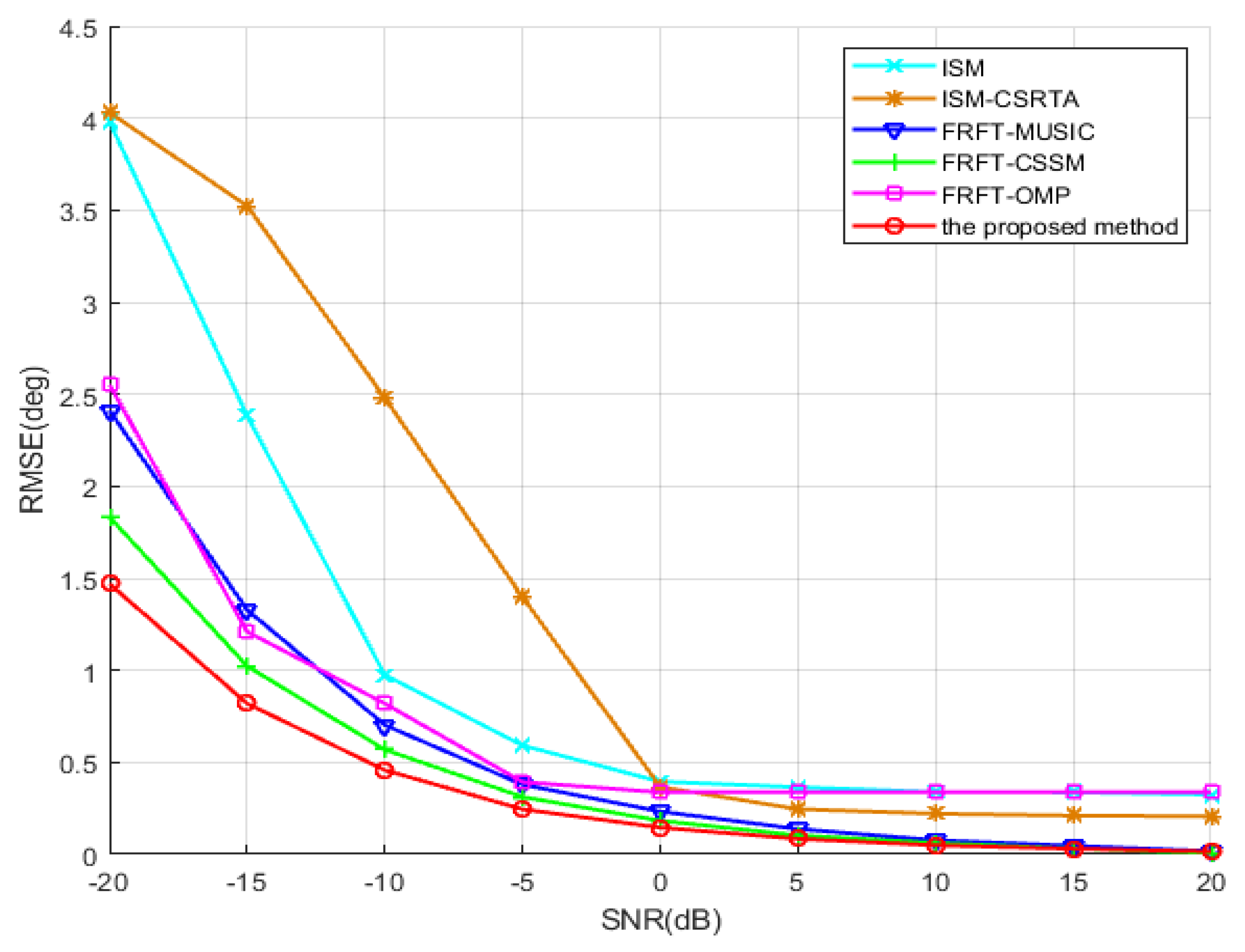
In the third simulation, the RMSE of the DOA estimations is compared in respect of different input SNRs, which vary from −20 to 20 dB with an interval of 5 dB. The number of snapshots is 1024. As shown in
Figure 8, the result illustrates that the DOA estimations by the proposed method become more and more accurate as SNR increases, and obviously outperform those by ISM, ISM-CSRTA, FRFT-MUSIC, FRFT-CSSM and FRFT-OMP approaches. Theoretically speaking, ISM-based algorithms decompose the wideband signals into several independent narrowband signals, and approximately assume that the frequency stays time-invariant in every frequency bin, without taking the continuous and linear time-varying characteristic of frequency and the whole wideband information into account. Moreover, they are based on the ULA or random array, and their DOFs are limited by the number of physical sensors. Hence, their accuracies of DOA estimation would be seriously affected. In view of a bigger aperture in the random array than that in the ULA, the RMSE of the ISM-CSRTA is slightly better than that of the ISM at high SNR. By contrast, the FRFT-based methods can estimate DOA of wideband LFM signals with time-variant frequency and steering vector, by transforming to time-invariant ones in FRF domain as shown in Equation (
15). The RMSE of DOA estimation by FRFT-MUSIC is improved, but still based on the ULA, which is also constrained by the number of physical sensors. FRFT-CSSM method selects the maximum contiguous part of the difference co-array and forms an ULA, which has more sensors than FRFT-MUSIC method, so its DOF is improved to a certain extent and its accuracy of DOA estimation is better than that of FRFT-MUSIC method. Nevertheless, this method gives up the information of the discontiguous part in the difference co-array, so its accuracy performance would be compromised. Although FRFT-OMP method adopts all sensors of the difference co-array to improve DOF, it is based on the CS framework. Because the discrete grids are pre-defined at several spatial directions, it inherently has the grid mismatch problem, which would significantly degrade the accuracy of DOA estimation especially when DOAs of signals deviate from the discrete grids. Moreover, it exploits discrete basis (such as
norm) to recover signal without noise, which is inevitable to bring substantial bias. In order to overcome the above shortcomings, in the proposed method, atomic norm minimization is adopted to reconstruct the covariance matrix, which has a continuous spatial parameter and effectively avoids the discrete grid mismatch problem. Moreover, the proposed method constructs a longer ULA by interpolating the virtual sensors, whose DOF is much bigger than that of the other algorithms. Therefore, the proposed method has a more accurate DOA estimation performance.
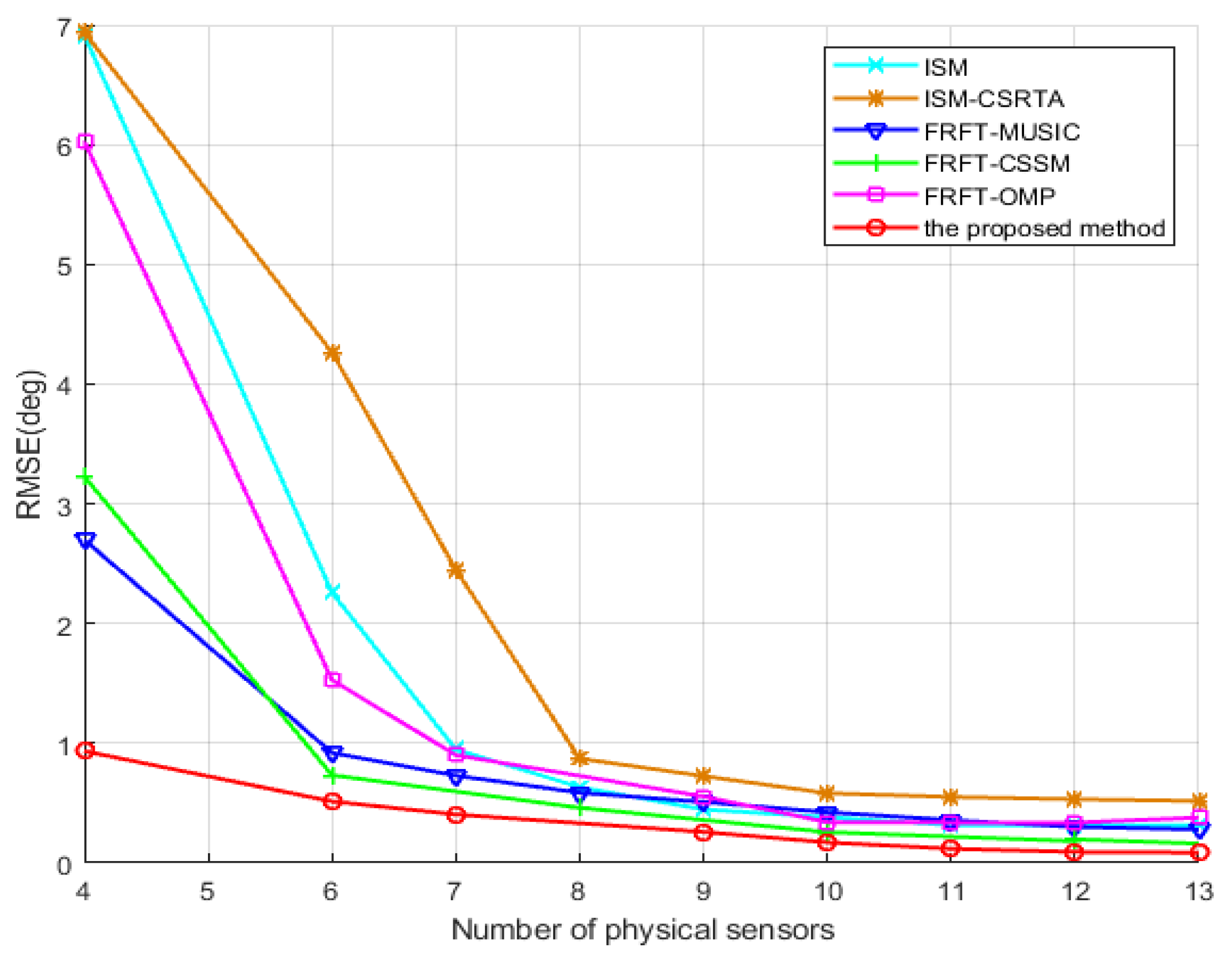
The fourth simulation further investigates the same scenario as the above one yet at a different number of physical sensors in the coprime array, which illustrates the influence of the number of physical sensors on accuracy. The number of physical sensors varies from 4 to 13 with SNR = −10 dB. As can be seen in
Figure 9, the proposed method improves the estimation performance as the number of physical sensors increases, and its RMSE is much smaller than that of ISM, ISM-CSRTA, FRFT-MUSIC, FRFT-CSSM and FRFT-OMP methods, especially with less physical sensors. As analysis in FTFT-MUSIC [
16], once the number of wideband sources remains the same, the smaller the number of physical sensors becomes, the bigger its RMSE is. Likewise, FRFT-CSSM employs the maximum contiguous ULA part of the difference co-array to increase available virtual sensors, but if the number of physical sensors decreases, the available virtual sensors would drastically reduce, and the RMSE would also become bigger. Although FRFT-OMP employs all the virtual sensors of the difference co-array to increase DOFs, the CS recovery approach would result in the grid mismatch and deviation from discrete grids. Furthermore, with the reduction of number of physical sensors, the number of virtual sensors in the difference co-array also declines sharply, which causes the accuracy of DOA estimation degrade severely. With the same number of physical sensors, the DOF of the proposed method is much bigger than that of the other methods. The result also shows that the accuracy of the proposed algorithm is significantly improved, which surpasses that of the other methods, especially with less sensors.
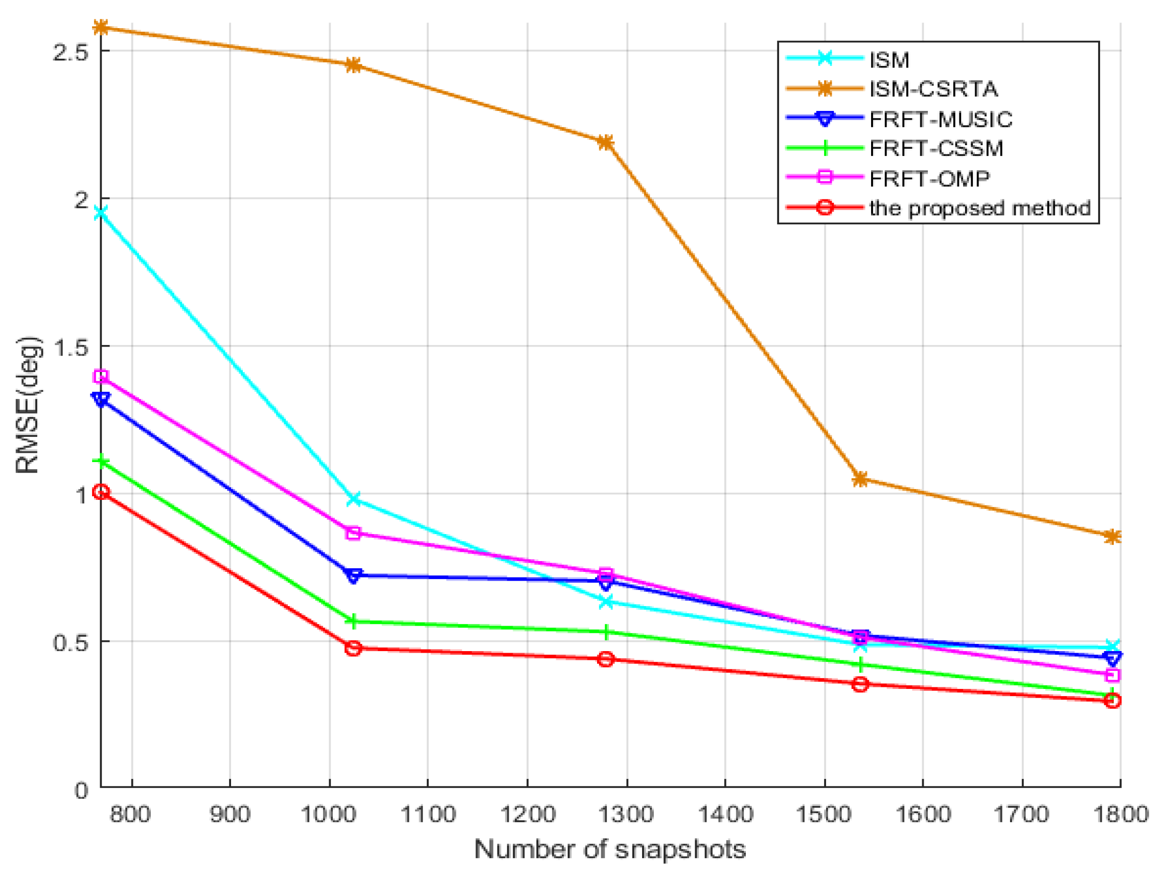
In the following, estimation accuracy of the proposed method with respect to the number of snapshots would be verified in the fifth simulation. The number of snapshots varies from 768 to 1792 with an interval of 256. The number of physical sensors is 7 in the coprime array and SNR = −10 dB. From
Figure 10, the result illustrates that RMSE of the DOA estimations by the proposed method becomes smaller and smaller as the number of snapshots increases, and is superior to that of ISM, ISM-CSRTA, FRFT-MUSIC, FRFT-CSSM and FRFT-OMP approaches once again.
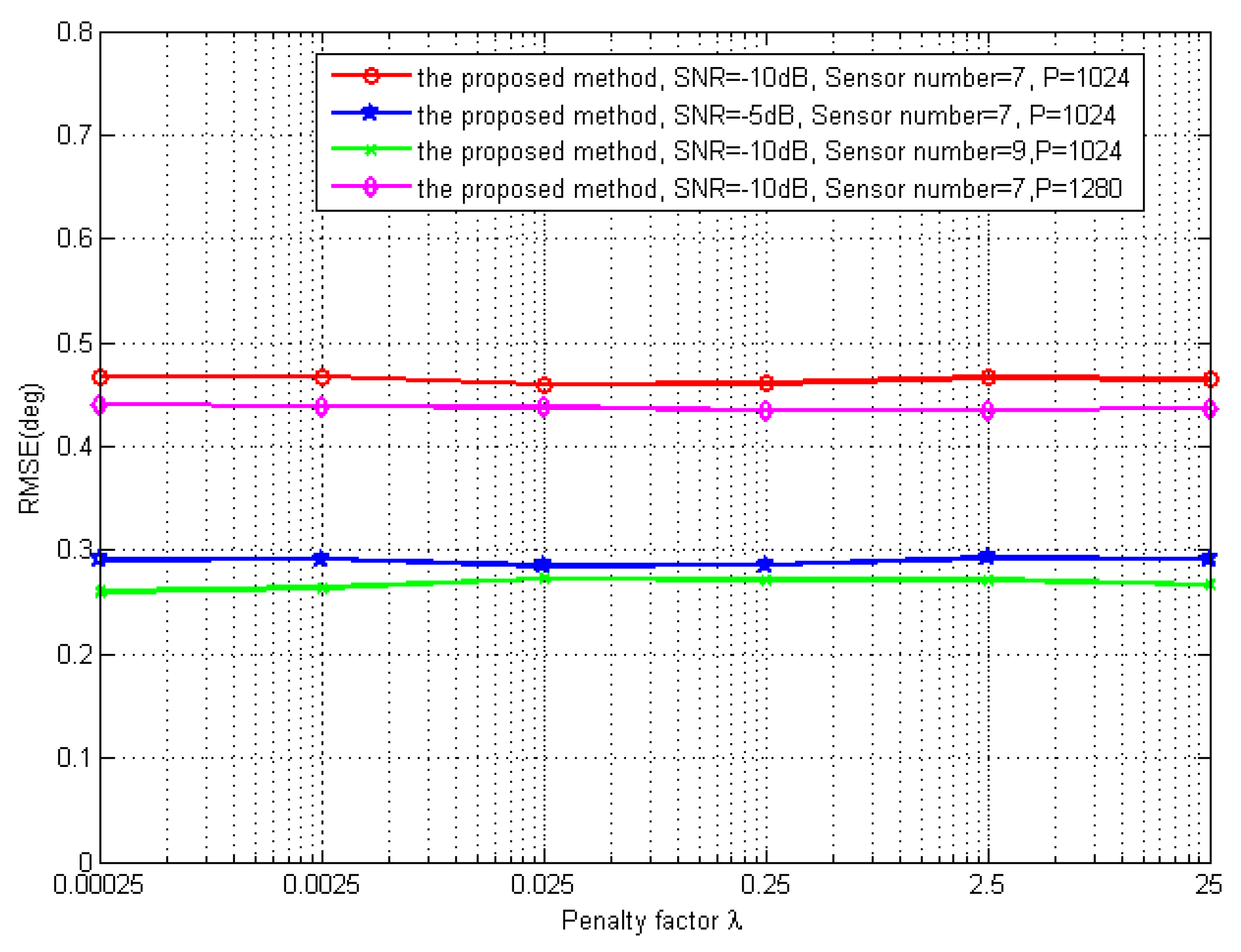
The sixth simulation discusses the influence of the penalty factor
. Consider the same scenario as the aforementioned ones yet at different penalty factors in optimization. In
Figure 11, it is evident that the RMSE remains the same while the penalty factor
increases from 0.00025 to 25, even with the different SNR, the number of physical sensors or the number of snapshots, respectively. The proposed method is robust with respect to the change of the penalty factor
. That is also the reason why we choose
= 0.25 in the simulation.
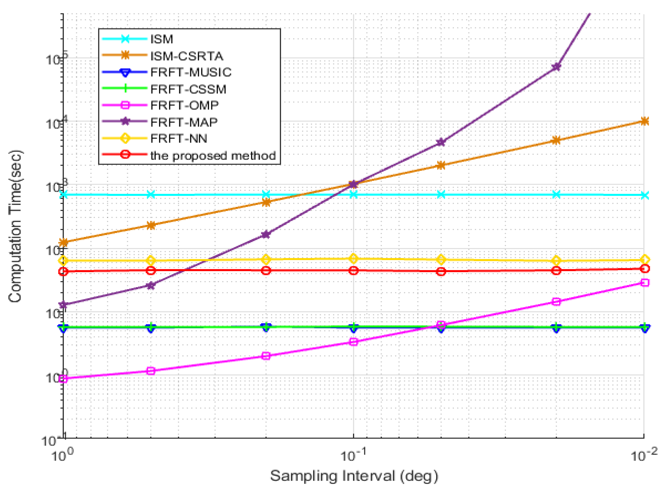
In the last simulation, the computational complexity measured by the computation time is verified for 100 Monte Carlo trials, which uses on a desktop with an Intel Core i7-7600U CPU. The sampling interval is varied from to
to
. In
Figure 12, it can be clearly observed that the computation times of the CS-based algorithms, such as ISM-CSRTA, FRFT-OMP and FRFT-MAP, increase when the grid intervals reduce and the pre-defined discrete grids become denser. However, the gridless DOA algorithms have nothing to do with the discrete grids, so they do not change with grid interval. Among them, ISM has a higher computational complexity than other gridless wideband DOA estimation algorithms, because it needs to estimate the DOA in every frequency bin and repeat this process in all frequency bins. The proposed method based on the continuous dictionary solves the optimization and recovers the sparse signals without the pre-defined discrete grids, so its computation time also has no connection with discrete grids and its sampling interval. Although it has slightly longer computation time than FRFT-MUSIC and FRFT-CSSM algorithms, it solves the underdetermined problem in wideband DOA estimation, which is insolvable by the other algorithms, and its DOF and estimation performance became better than the other wideband DOA algorithms.


