Object-Level Double Constrained Method for Land Cover Change Detection


Abstract
:1. Introduction
2. Materials and Methods
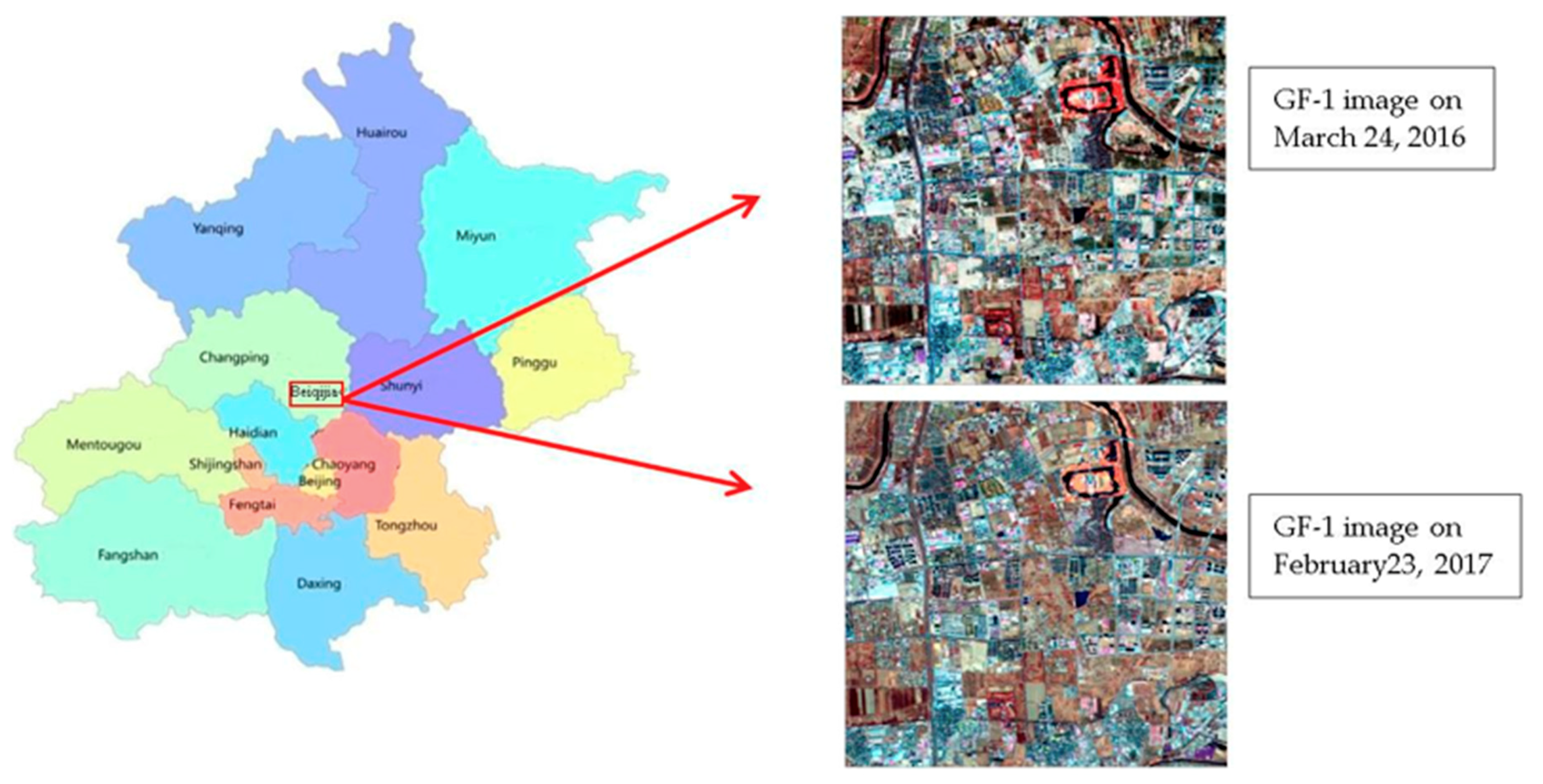
2.1. Materials
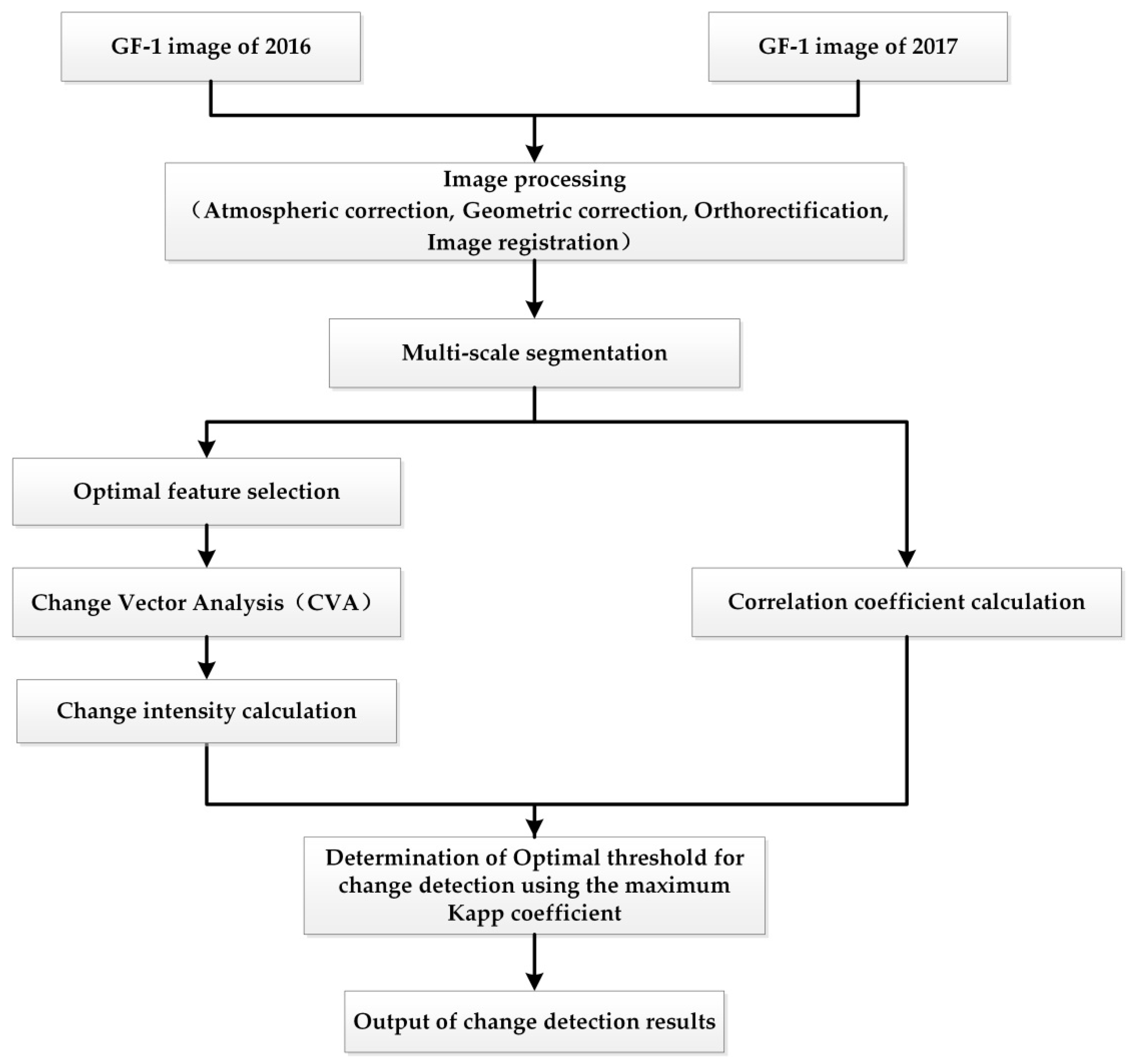
2.2. Methods
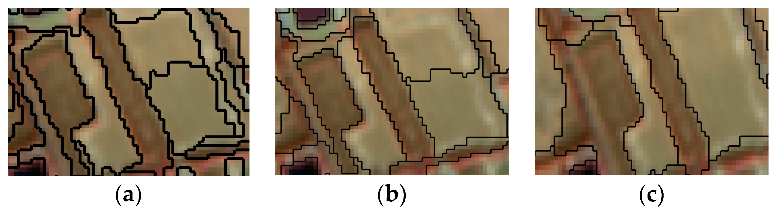
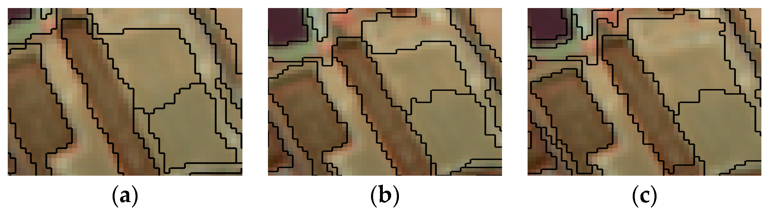
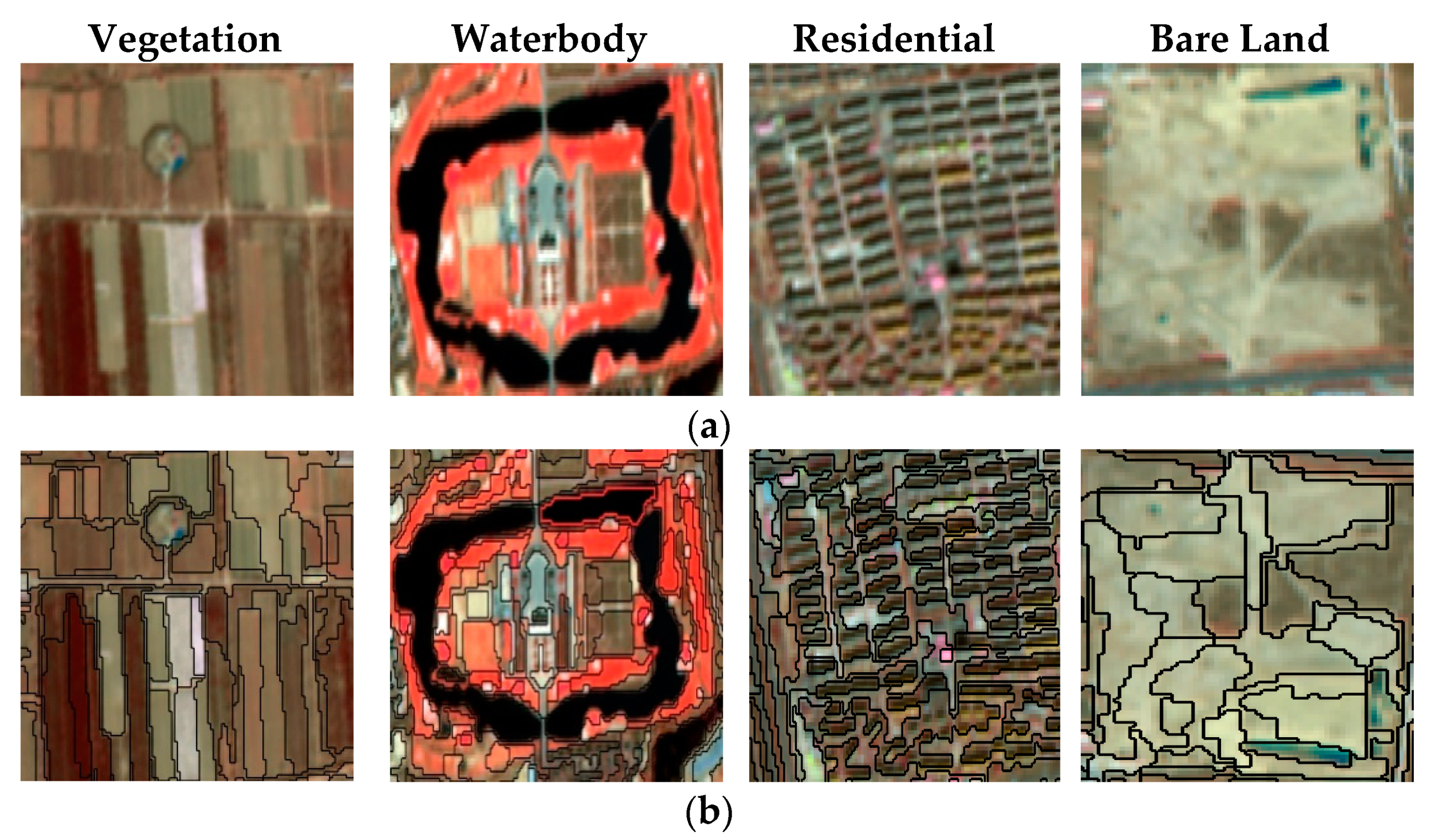
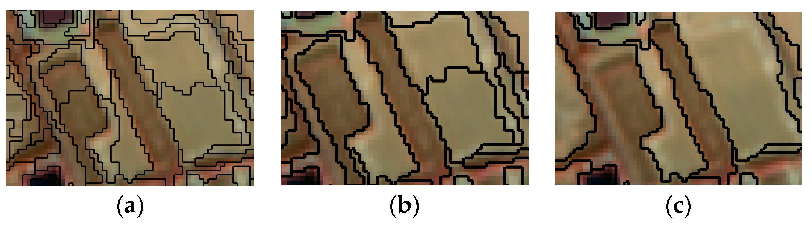
2.2.1. Multi-Scale Segmentation
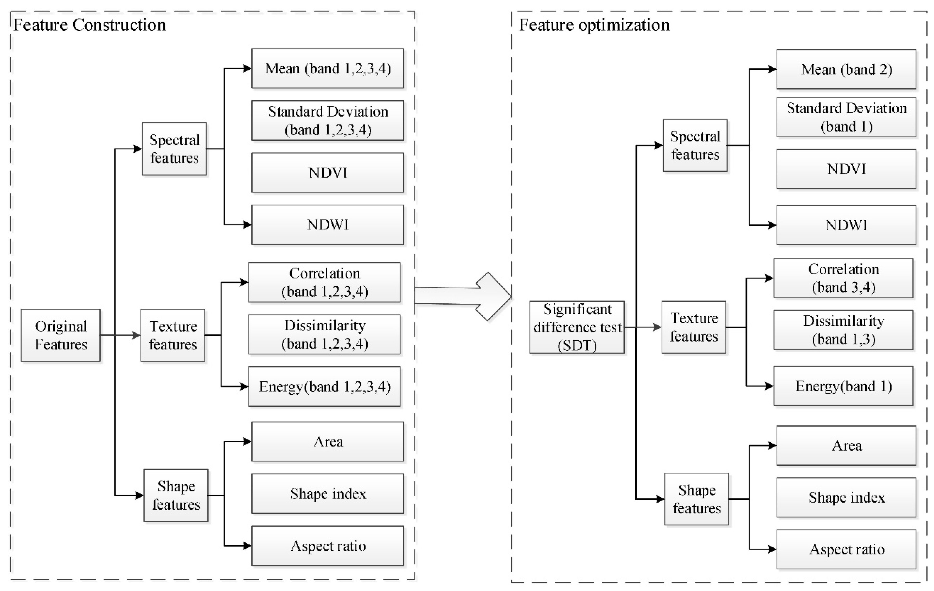
2.2.2. Optimal Feature Selection
Feature Construction
Feature Selection
2.2.3. Change Vector Analysis
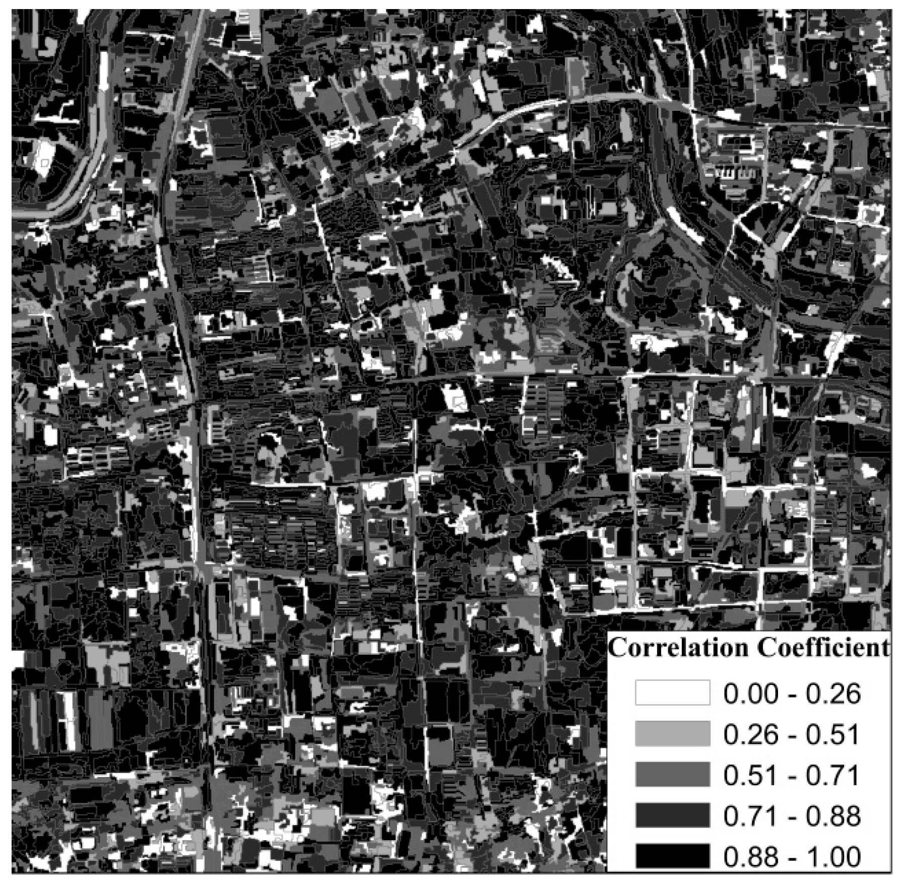
2.2.4. Correlation Coefficient Calculation
2.2.5. Optimal Threshold Determination for Change Detection
3. Results and Discussion
3.1. Multi-Scale Segmentation
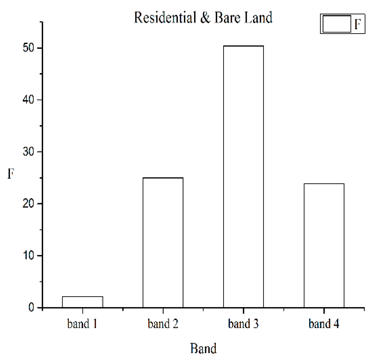
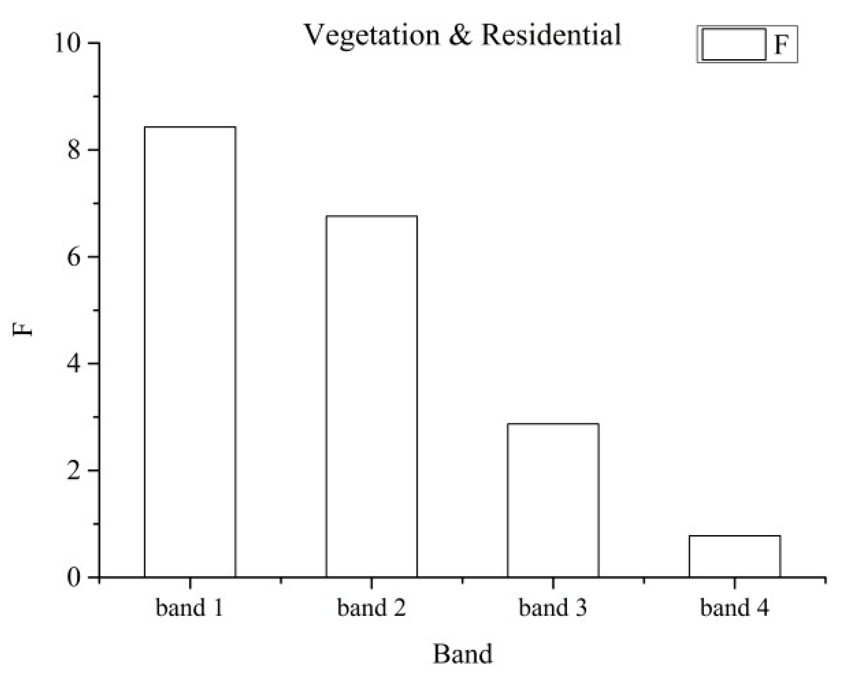
3.2. Optimal Feature Selection
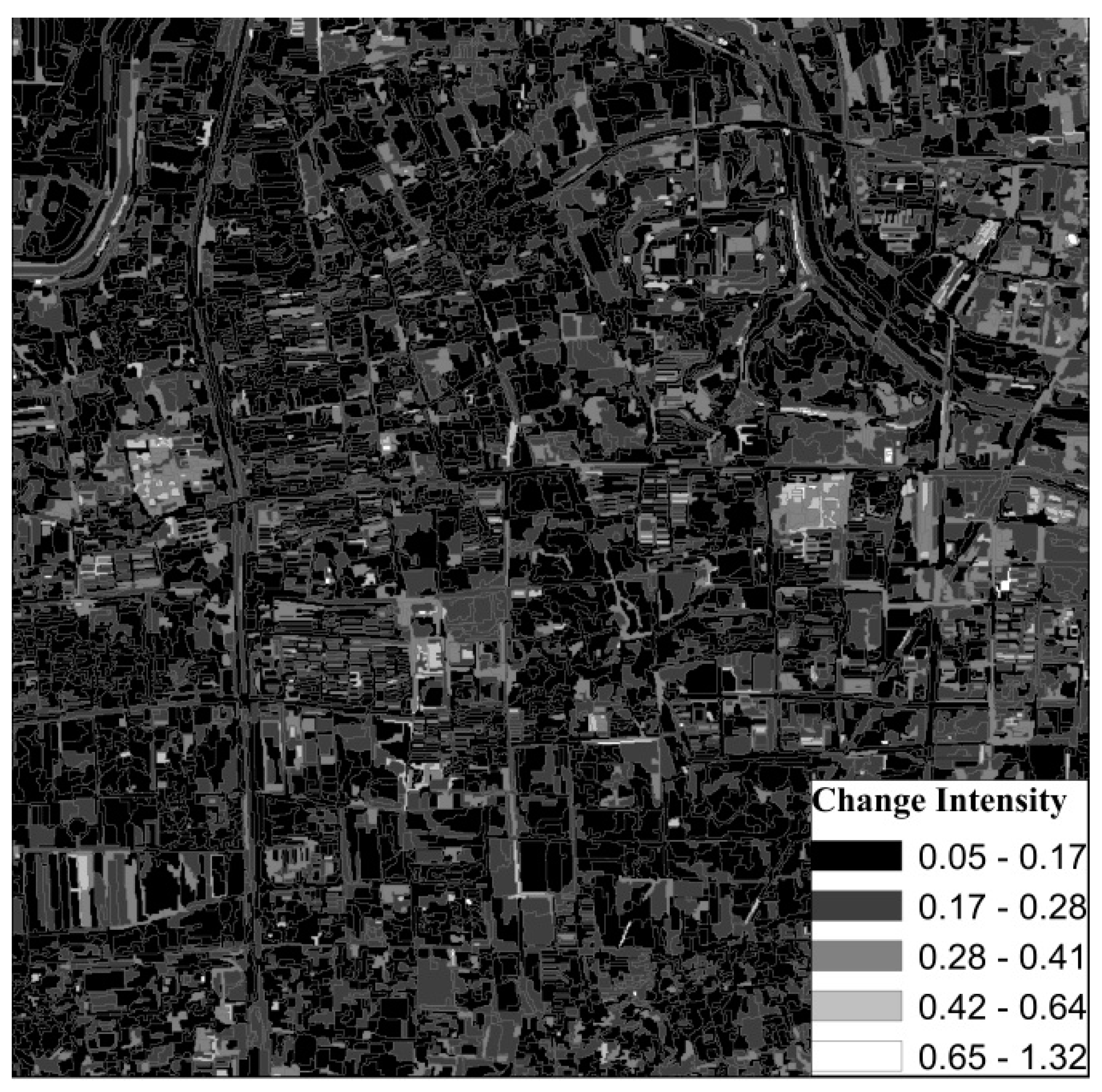
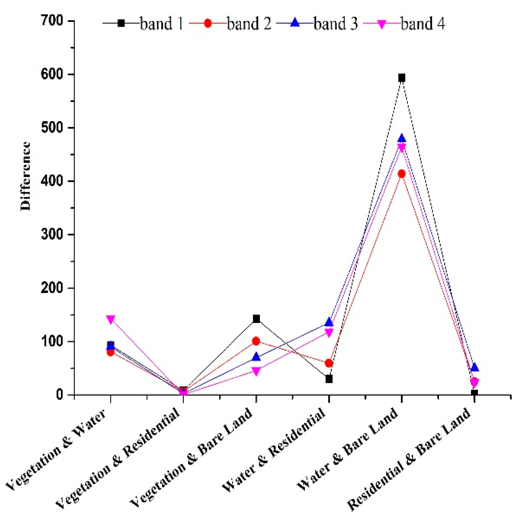
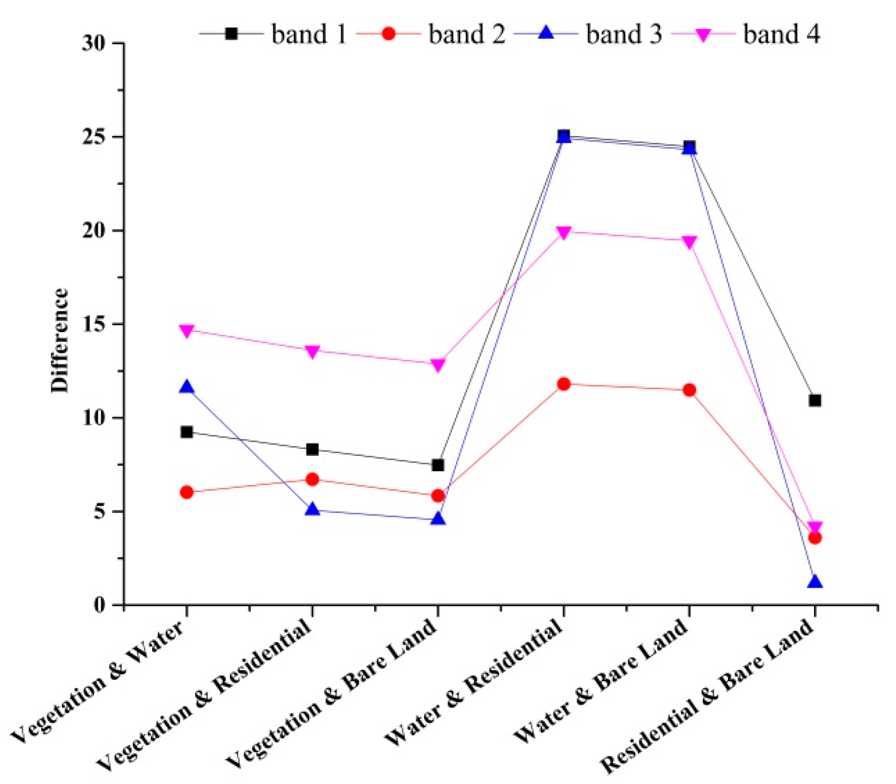
3.3. Change Intensity and the Correlation Coefficient
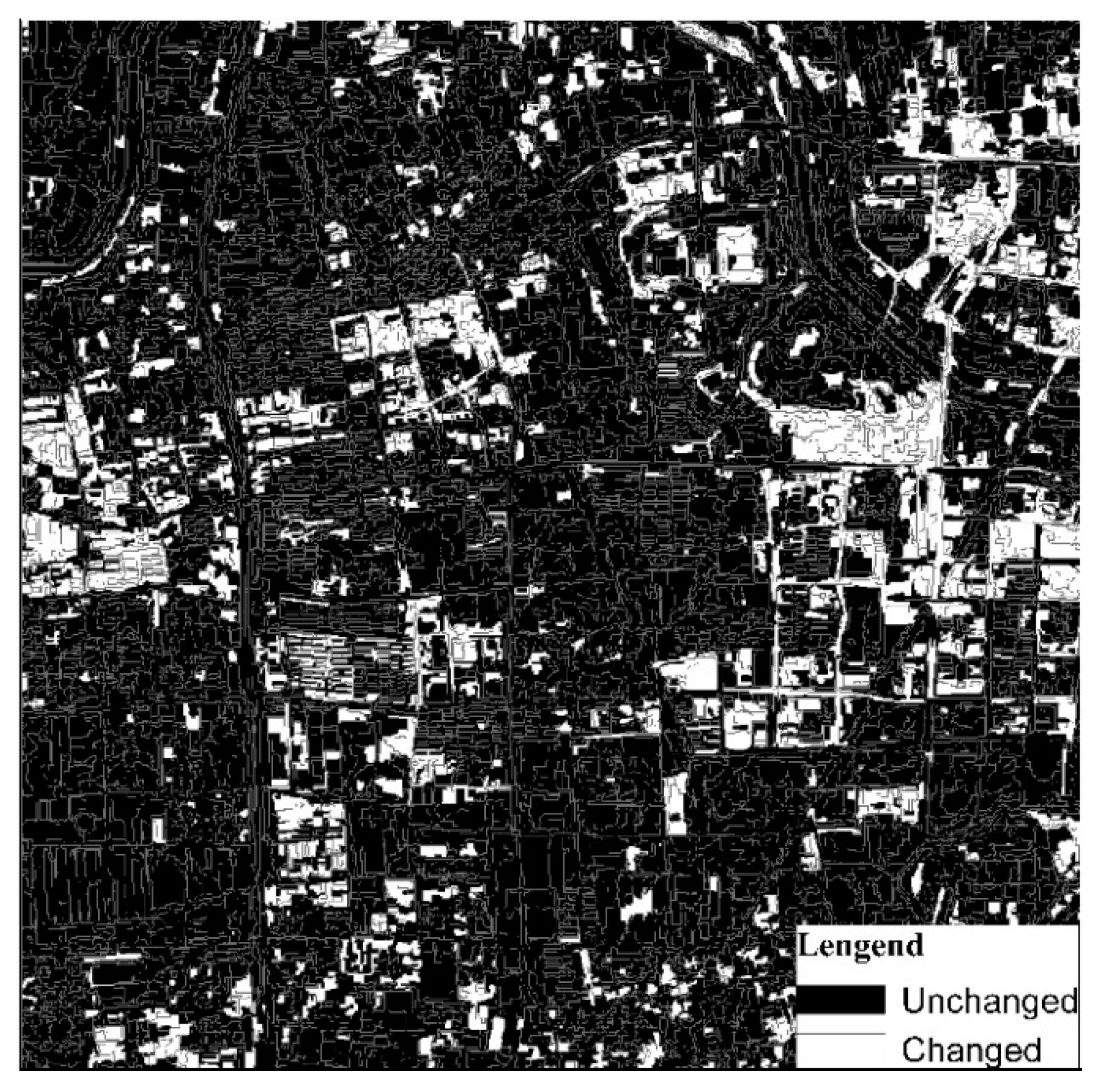
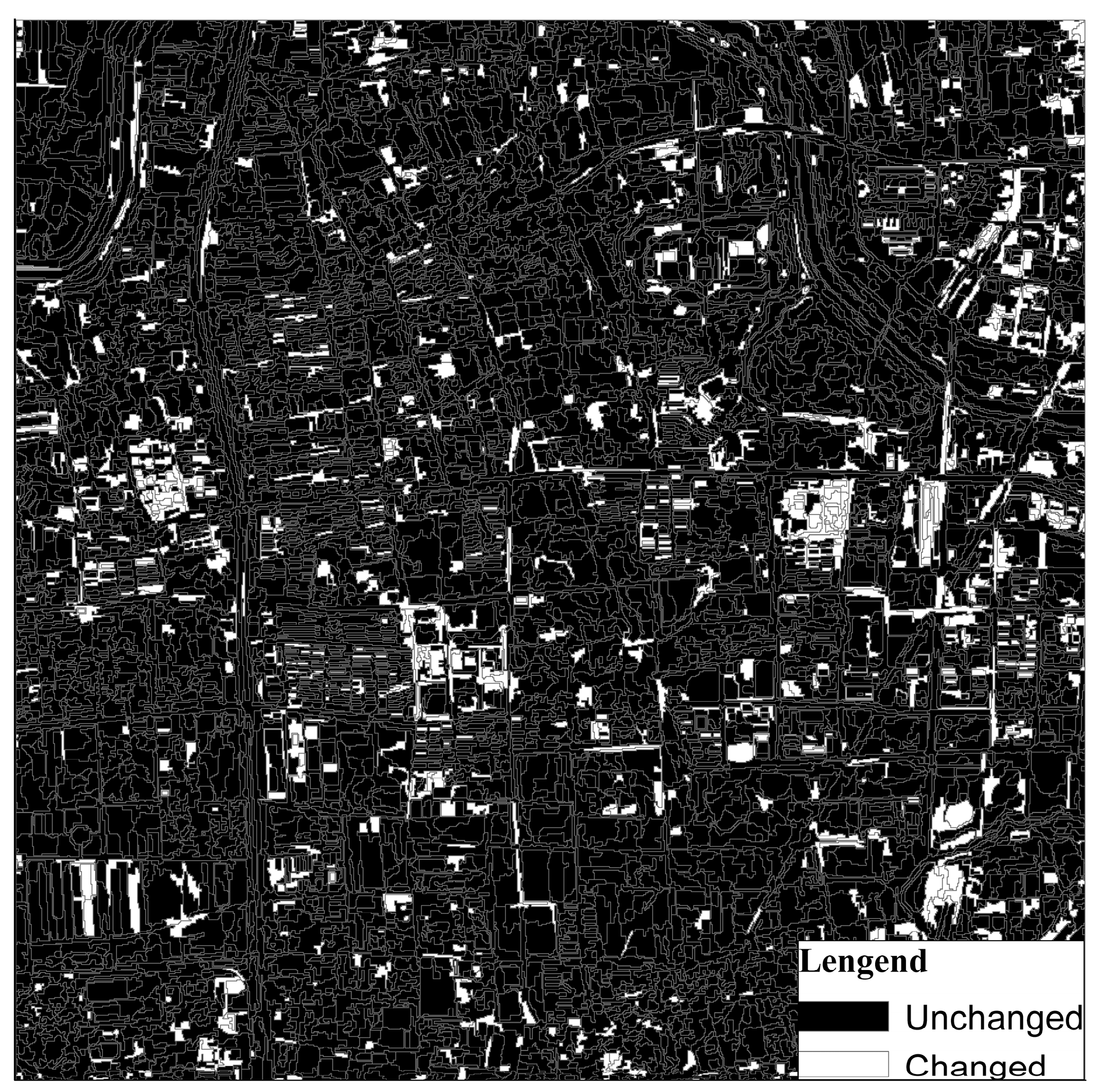
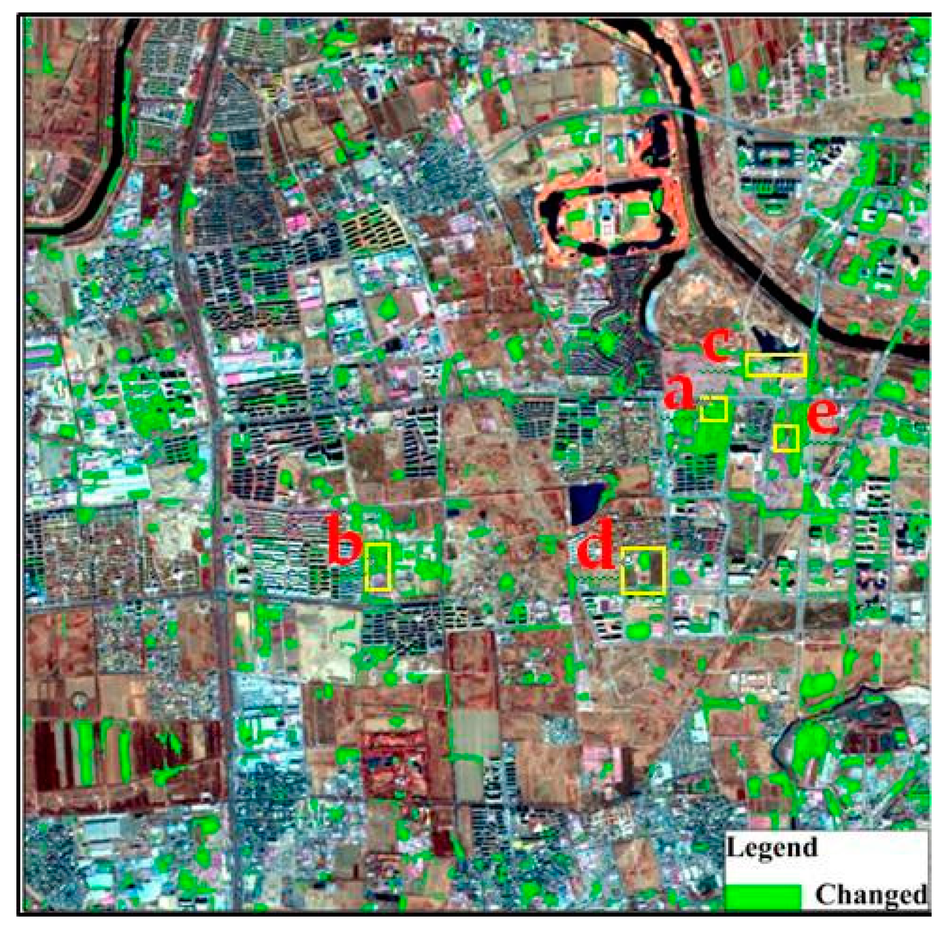
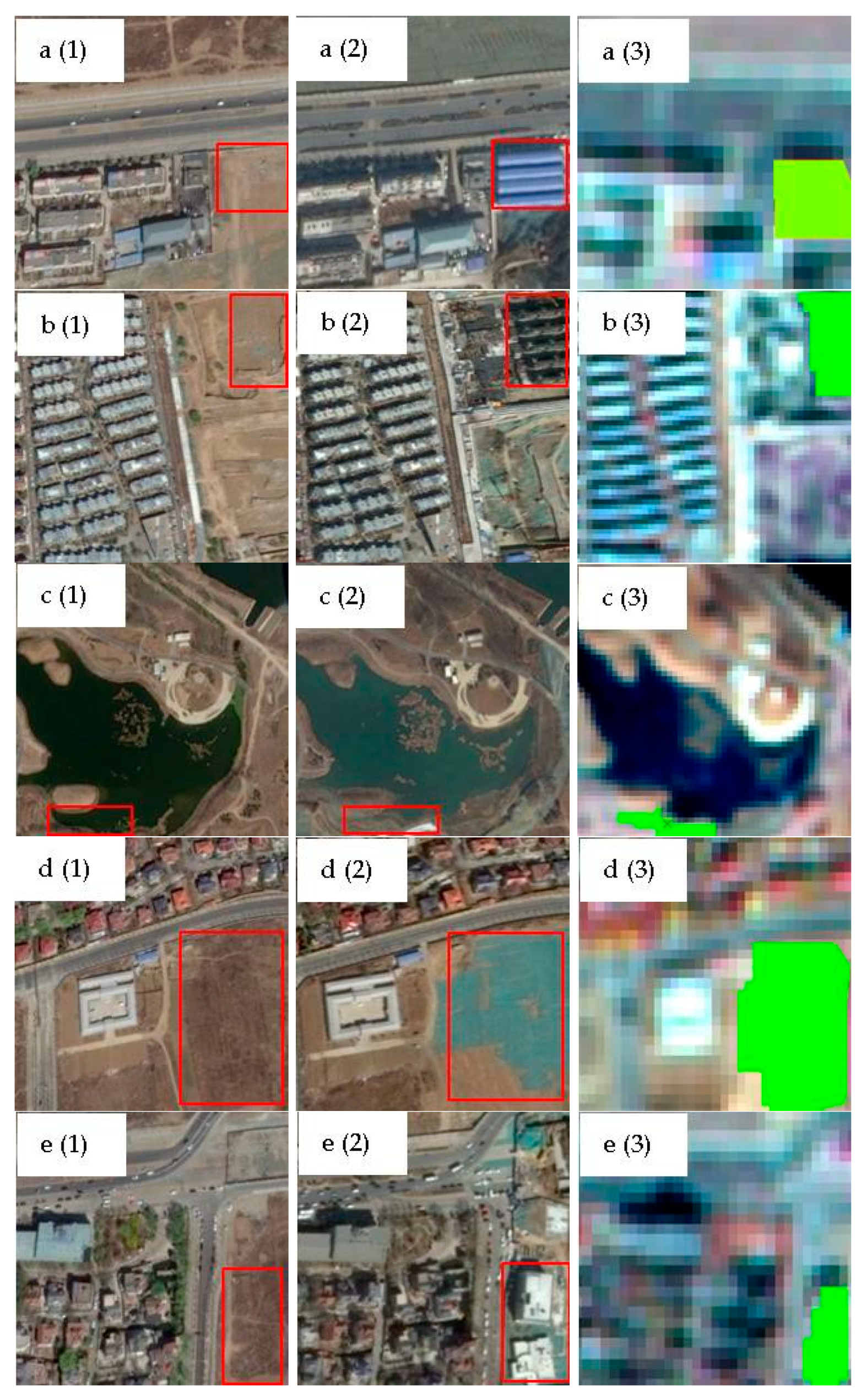
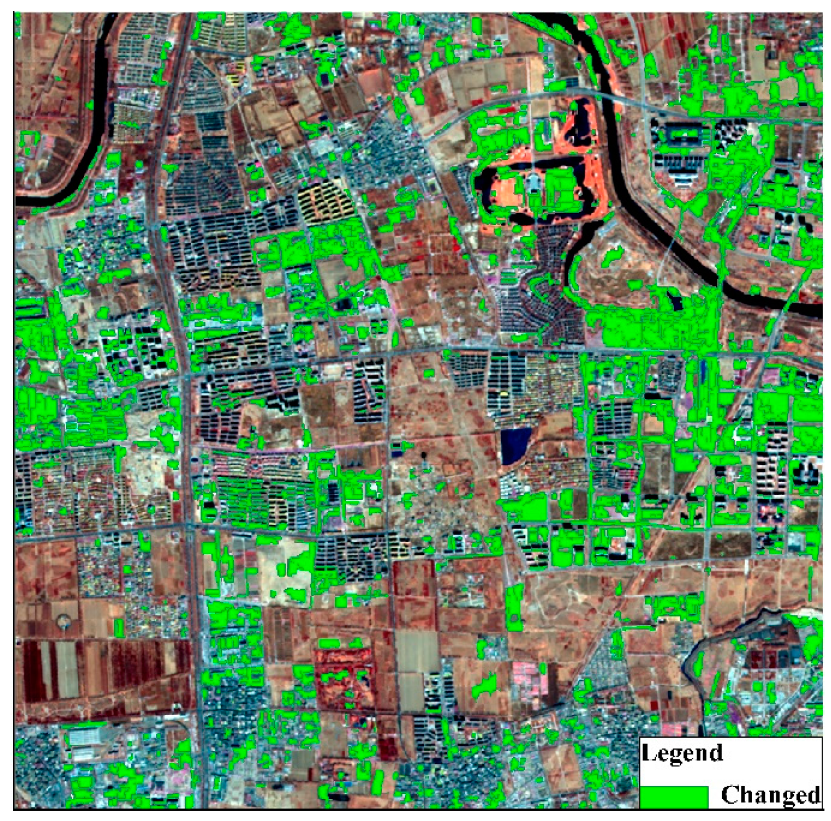
3.4. Land Cover Change Detection
3.4.1. Results from SCCD
3.4.2. Results from the ODCD
3.5. Precision Comparison
4. Conclusions
- (1)
- Combining change vector analysis with correlation coefficients based on object-level, the ODCD can reduce the shortcomings of seasonal sensitivity of SCCD and improve the accuracy of land cover change detection. The ODCD’s overall accuracy was 92.19% and this was 10% higher than that of SCCD. At the same time, its overall error was 20% and it was 27% lower than that of SCCD.
- (2)
- ODCD can be used to reduce the number of features and improve the computational efficiency. The SDT is an effective feature optimization method. Using optimal feature selection, the feature dimensions were reduced from 26 to 12, which increased the calculation speed.
Author Contributions
Funding
Acknowledgments
Conflicts of Interest
References
- Sun, Q.; Zhang, X.; Zhang, H.; Niu, H. Coordinated development of a coupled social economy and resource environment system: A case study in Henan Province, China. Environ. Dev. Sustain. 2018, 20, 1385–1404. [Google Scholar] [CrossRef]
- Yue, W.Z.; Xu, J.H.; Xu, L.H. An analysis on eco-environmental effect of urban land use based on remote sensing images: a case study of urban thermal environment and ndvi. Acta Ecol. Sin. 2006, 26, 1450–1460. [Google Scholar] [CrossRef]
- Liverman, D.; Moran, E.F.; Rindfuss, R.R. People and Pixels: Linking Remote Sensing and Social Science; National Academies Press: Washington DC, USA, 1998; pp. 362–363. [Google Scholar] [CrossRef]
- Yuan, D.; Elvidge, C. NALC Land Cover Change Detection Pilot Study: Washington, D.C. Area Experiments. Remote Sens. Environ. 1998, 66, 166–178. [Google Scholar] [CrossRef]
- Johnson, R.D.; Kasischke, E.S. Change vector analysis: A technique for the multispectral monitoring of land cover and condition. Int. J. Remote Sens. 2006, 19, 411–426. [Google Scholar] [CrossRef]
- Zhou, B. The research on land use change detection by using direct classification of stacked multitemporal TM images. J. Nat. Resour. 2001, 16, 263–268. [Google Scholar] [CrossRef]
- Li, X.; Yeh, A.G.O. Application of remote sensing for monitoring and analysis of urban expansion: A case study of Dongguan. Geogr. Res. 1997, 16, 1450–1460. [Google Scholar] [CrossRef]
- Li, X.; Shu, N.; Yang, J.; Li, L. The land-use change detection method using object-based feature consistency analysis. In Proceedings of the 2011 19th International Conference on Geoinformatics, Shanghai, China, 24–26 June 2011; pp. 1–6. [Google Scholar] [CrossRef]
- Im, J.; Jensen, J.R.; Tullis, J.A. Object-based change detection using correlation image analysis and image segmentation. Int. J. Remote Sens. 2008, 29, 399–423. [Google Scholar] [CrossRef]
- Lobo, A.; Chic, O.; Casterad, A. Classification of Mediterranean crops with multisensor data: Per-pixel versus per-object statistics and image segmentation. Int. J. Remote Sens. 1996, 17, 2385–2400. [Google Scholar] [CrossRef]
- Wang, W.J.; Zhao, Z.M.; Zhu, H.Q. Object-oriented multi-feature fusion change detection method for high resolution remote sensing image. In Proceedings of the 2009 17th International Conference on Geoinformatics, Fairfax, VA, USA, 12–14 August 2009. [Google Scholar] [CrossRef]
- Lu, D.; Hetrick, S.; Moran, E.; Li, G. Detection of urban expansion in an urban-rural landscape with multitemporal Quick Bird images. J. Appl. Remote Sens. 2010, 4, 201–210. [Google Scholar] [CrossRef]
- Hussain, E.; Shan, J. Object-based urban land cover classification using rule inheritance over very high-resolution multisensor and multitemporal data. Mapp. Sci. Remote Sens. 2016, 53, 164–182. [Google Scholar] [CrossRef]
- Zhou, Q.M. Review on Change Detection Using Multi-temporal Remotely Sensed Imagery. Acta Ecol. Sin. 2011, 2, 28–33. [Google Scholar]
- Zhao, M.; Zhao, Y.D. Object -oriented and multi-feature hierarchical change detection based on CVA for high-resolution remote sensing imagery. Acta Ecol. Sin. 2018, 22, 119–131. [Google Scholar] [CrossRef]
- Quarmby, N.A.; Townshend, J.R.G. Preliminary analysis of SPOT HRV multispectral products of an arid environment. Int. J. Remote Sens. 1986, 7, 1869–1877. [Google Scholar] [CrossRef]
- Fan, H.; Ainai, M.A.; Jing, L.I. Case Study on Image Differencing Method for Land Use Change Detection Using Thematic Data in Renhe District of Panzhihua. J. Remote Sens. 2001, 5, 75–80. [Google Scholar]
- Li, X.; Yeh, A.G.O. Accuracy Improvement of Land Use Change Detection Using Principal Components Analysis: A Case Study in the Pearl River Delta. J. Remote Sens. 1997, 1, 283–288. [Google Scholar]
- Yuanyong, D.; Fang, S.; Yao, C. Change detection for high-resolution images using multilevel segment method. Acta Ecol. Sin. 2016, 20, 129–137. [Google Scholar] [CrossRef]
- Yu, X.F.; Luo, Y.Y.; Zhuang, D.F.; Wang, S.K.; Wang, Y. Comparative analysis of land cover change detection in an Inner Mongolia grassland area. Acta Ecol. Sin. 2014, 34, 7192–7201. [Google Scholar] [CrossRef]
- Qi, Z.; Yeh, A.G.O.; Li, X.; Zhang, X. A three-component method for timely detection of land cover changes using polarimetric SAR images. J. Photogramm. Remote Sens. 2015, 107, 3–21. [Google Scholar] [CrossRef]
- Wang, L.; Yan, L.I.; Wang, Y. Research on Land Use Change Detection Based on an Object-oriented Change Vector Analysis Method. J. Geo-Inf. Sci. 2014, 27, 74–80. [Google Scholar] [CrossRef]
- Chen, J.; Chun-Yang, H.E.; Zhuo, L. Land Use/Cover Change Detection with Change Vector Analysis (CVA): Change Type Determining. J. Remote Sens. 2001, 5, 346–352. [Google Scholar]
- Lambin, E.F.; Strahler, A.H. Change-vector analysis in multitemporal space: a tool to detect and categorize land-cover change processes using high temporal-resolution satellite data. Remote Sens. Environ. 1994, 48, 231–244. [Google Scholar] [CrossRef]
- Ling, O.; Mao, D.; Wang, Z.; Li, H.; Man, W.; Jia, M.; Liu, M.; Zhang, M.; Liu, H. Analysis crops planting structure and yield based on GF-1 and Landsat8 OLI images. Trans. Chin. Soc. Agric. Eng. 2017, 33, 147–156. [Google Scholar] [CrossRef]
- Fan, J.; Zhao, D.; Wang, J. Oil spill GF-1 remote sensing image segmentation using an evolutionary feed forward neural network. In International Joint Conference on Neural Networks. In Proceedings of the 2014 International Joint Conference on Neural Networks (IJCNN), Beijing, China, 6–11 July 2014; pp. 460–464. [Google Scholar]
- Cohen, J. A Coefficient of Agreement for Nominal Scales. Educ. Psychol. Meas. 1960, 20, 37–46. [Google Scholar] [CrossRef]
- Cohen, J. Weighted kappa: Nominal scale agreement provision for scaled disagreement or partial credit. Psychol. Bull. 1968, 70, 213–220. [Google Scholar] [CrossRef]
- Wei, S.U.; Jing, L.I.; Chen, Y.H.; Zhang, J.S.; Hu, D.Y.; Low, T.M. Object-oriented Urban Land-cover Classification of Multi-scale Image Segmentation Method—A Case Study in Kuala Lumpur City Center, Malaysia. J. Remote Sens. 2007, 11, 521–530. [Google Scholar]
- Zhiwei, Q. Object-oriented Multi-scale Segmentation Algorithm for Remote Sensing Image. Geospat. Inf. 2013, 11, 95–96. [Google Scholar] [CrossRef]
- Ma, H.R. Object-Based Remote Sensing Image Classification of Forest Based on Multi-Level Segmentation; Beijing Forestry University: Beijing, China, 2014. [Google Scholar]
- Zhuang, H.; Deng, K.; Fan, H.; Yu, M. Strategies Combining Spectral Angle Mapper and Change Vector Analysis to Unsupervised Change Detection in Multispectral Images. IEEE Geosci. Remote Sens. Lett. 2016, 13, 681–685. [Google Scholar] [CrossRef]
- Wu, X.H. The Studies on Land Cover Change Detection Based on Object-Oriented Method; Henan University of Technology: Zhengzhou, Henan, China, 2013. [Google Scholar]
- Zhang, Z.J.; Li, A.N.; Lei, G.B.; Bian, J.H.; Wu, B.F. Change detection of remote sensing images based on multiscale segmentation and decision tree algorithm over mountainous area: A case study in Panxi region, Sichuan Province. Acta Ecol. Sin. 2014, 34, 7222–7232. [Google Scholar] [CrossRef]
- Haralick, R.M.; Shanmugam, K.; Dinstein, I. Textural Features for Image Classification. IEEE Trans. Syst. Man Cybern. 1973, 6, 610–621. [Google Scholar] [CrossRef]
- Wu, Z.; Zeng, J.X.; Gao, Q.Q. Aircraft target recognition in remote sensing images based on saliency images and multi-feature combination. J. Image Graph. 2017, 22, 532–541. [Google Scholar] [CrossRef]
- Brunsdon, C.; Fotheringham, A.S.; Charlton, M. Some Notes on Parametric Significance Tests for Geographically Weighted Regression. J. Reg. Sci. 2010, 39, 497–524. [Google Scholar] [CrossRef]
- Statistical Processing and Explanation of GB/T. 4883-2008; Standardization Administration of the PRC: Beijing, China, 2008.
- Malila, W.A. Change Vector Analysis: An Approach for Detecting Forest Changes with Landsat. Available online: http://citeseerx.ist.psu.edu/viewdoc/download?doi=10.1.1.462.1459&rep=rep1&type=pdf (accessed on 26 December 2018).
- Pyle, D. Data Preparation for Data Mining; Morgan Kaufmann Publishers: San Francisco, CA, USA, 1999; pp. 375–381. ISBN 9781558605299. [Google Scholar]
- Jain, A.K.; Duin, R.P.W.; Mao, J. Statistical pattern recognition: A review. IEEE Trans. Pattern Anal. Mach. Intell. 2000, 22, 4–37. [Google Scholar] [CrossRef]
- Fung, T.; Ledrew, E.F. The Determination of Optimal Threshold Levels for Change Detection Using Various Accuracy Indices. Photogramm. Eng. Remote Sens. 1988, 54, 1449–1454. [Google Scholar]
- Van Oort, P.A.J. Interpreting the change detection error matrix. Remote Sens. Environ. 2007, 108, 1–8. [Google Scholar] [CrossRef]
- Neuhäuser, M. Markus: Two-sample tests when variances are unequal. Anim. Behav. 2002, 63, 823–825. [Google Scholar] [CrossRef]


| Feature Parameters | Formula | Formula Description |
|---|---|---|
| Mean | is the sum of all pixel values divided by the total number of pixels in one object. | |
| Standard deviation | is the value of all pixels in the object, is the mean of the object. | |
| NDVI | is the reflectance for the near-infrared band, is the reflectance for the infrared band. | |
| NDWI | is the reflectance of the green band, and is the reflectance of the near-infrared band. |
| Features Parameters | Formula | Formula Description |
|---|---|---|
| Correlation | i is the gray value of any point in the image; j is the gray value of another point deviating from the point; is the frequency of occurrence of the gray pair in the gray level co-occurrence matrix, and represent the mean values in the row and column direction, respectively, and and represent the variance in the row and column direction, respectively. It reflects the consistency of image texture and the degree of similarity of metric co-occurrence matrix elements in the row or column direction. | |
| Dissimilarity | is the frequency of occurrence of the gray pair in the gray level co-occurrence matrix. The higher the local contrast, the higher the similarity. | |
| Energy | is the frequency of occurrence of the gray pair in the gray level co-occurrence matrix. Energy is also called “the angle second moment.” When the image is a homogeneous area with a consistent texture, its energy is greater. |
| Feature Parameters | Formula | Formula Description |
|---|---|---|
| Area | is the value of pixel i. This describes the size of the object. For non-geographically referenced data, the area of the pixel is 1. | |
| Aspect ratio | S is the covariance matrix composed of the coordinates of points after object vectorization, w is the width, and is the length of each object. | |
| Shape index | The variable p is the perimeter of the image object, A is the area of the image object. This describes the compactness of an object. The higher the compactness, the greater the density, and the more similar the shape is to a square. |
| Assessment Data | ||||
|---|---|---|---|---|
| Unchanged | Changed | Total | ||
| Test results | Unchanged | |||
| Changed | ||||
| Total | ||||
| Verification Samples | Total | User Accuracy (%) | |||
|---|---|---|---|---|---|
| Unchanged | Changed | ||||
| Test Results | Unchanged | 121 | 5 | 126 | 96.03 |
| Changed | 15 | 72 | 87 | 82.70 | |
| Total | 136 | 77 | 213 | ||
| Producer Accuracy (%) | 88.97 | 93.50 | |||
| Verification Samples | Total | User Accuracy (%) | |||
|---|---|---|---|---|---|
| Unchanged | Changed | ||||
| Test Results | Unchanged | 122 | 8 | 130 | 93.85 |
| Changed | 5 | 78 | 83 | 93.98 | |
| Total | 127 | 86 | 213 | ||
| Producer Accuracy (%) | 96.06 | 90.70 | |||
| Verification Samples | Total | User Accuracy (%) | |||
|---|---|---|---|---|---|
| Unchanged | Changed | ||||
| Test Results | Unchanged | 172 | 28 | 200 | 86.00 |
| Changed | 32 | 101 | 133 | 75.94 | |
| Total | 204 | 129 | 333 | ||
| Producer Accuracy (%) | 84.31 | 78.29 | |||
| Verification Samples | Total | User Accuracy (%) | |||
|---|---|---|---|---|---|
| Unchanged | Changed | ||||
| Results | Unchanged | 186 | 14 | 200 | 93.00 |
| Changed | 12 | 121 | 133 | 90.98 | |
| Total | 198 | 135 | 333 | ||
| Producer Accuracy (%) | 93.94 | 89.63 | |||
| Overall Accuracy | Kappa Coefficient | Total Error | ||
|---|---|---|---|---|
| Misjudgment Error | Omission Error | |||
| SCCD | 81.98% | 0.62 | 24% | 22% |
| ODCD | 92.19% | 0.84 | 9% | 10% |
| Unchanged | Changed | Total | |
|---|---|---|---|
| Unchanged | 73 | 16 | 89 |
| Changed | 4 | 28 | 32 |
| Total | 77 | 44 | 121 |
| Unchanged | Changed | Total | |
|---|---|---|---|
| Unchanged | 83 | 6 | 89 |
| Changed | 4 | 28 | 32 |
| Total | 87 | 34 | 121 |
| Overall Accuracy | Kappa Coefficient | |
|---|---|---|
| SCCD | 83.66% | 0.62 |
| ODCD | 91.73% | 0.80 |
| Overall Accuracy Difference | Kappa Coefficient Difference | |
|---|---|---|
| Training group | 3.29% | 0.07 |
| Verification group 1 | 10.21% | 0.18 |
| Verification group 2 | 8.07% | 0.22 |
| p value | 0.03186 | 0.02286 |
© 2018 by the authors. Licensee MDPI, Basel, Switzerland. This article is an open access article distributed under the terms and conditions of the Creative Commons Attribution (CC BY) license (http://creativecommons.org/licenses/by/4.0/).
Share and Cite
Wang, Z.; Liu, Y.; Ren, Y.; Ma, H. Object-Level Double Constrained Method for Land Cover Change Detection. Sensors 2019, 19, 79. https://doi.org/10.3390/s19010079
Wang Z, Liu Y, Ren Y, Ma H. Object-Level Double Constrained Method for Land Cover Change Detection. Sensors. 2019; 19(1):79. https://doi.org/10.3390/s19010079
Chicago/Turabian StyleWang, Zhihao, Yalan Liu, Yuhuan Ren, and Haojie Ma. 2019. "Object-Level Double Constrained Method for Land Cover Change Detection" Sensors 19, no. 1: 79. https://doi.org/10.3390/s19010079
APA StyleWang, Z., Liu, Y., Ren, Y., & Ma, H. (2019). Object-Level Double Constrained Method for Land Cover Change Detection. Sensors, 19(1), 79. https://doi.org/10.3390/s19010079