Multi-Type Sensor Placements in Gaussian Spatial Fields for Environmental Monitoring †
Abstract
1. Introduction
2. Problem Formulation
2.1. Gaussian Process
2.2. Informative Locations for Single Spatial Field
2.3. Optimal Multi-Type Sensor Placement
3. Solution Approach
3.1. One-with-All Case
| Algorithm 1 Multi-type sensor deployment algorithm for one-with-all case |
|
3.2. General Case
| Algorithm 2 Multi-type sensor deployment algorithm for the general cost case |
|
3.3. Assessing the Trade Off
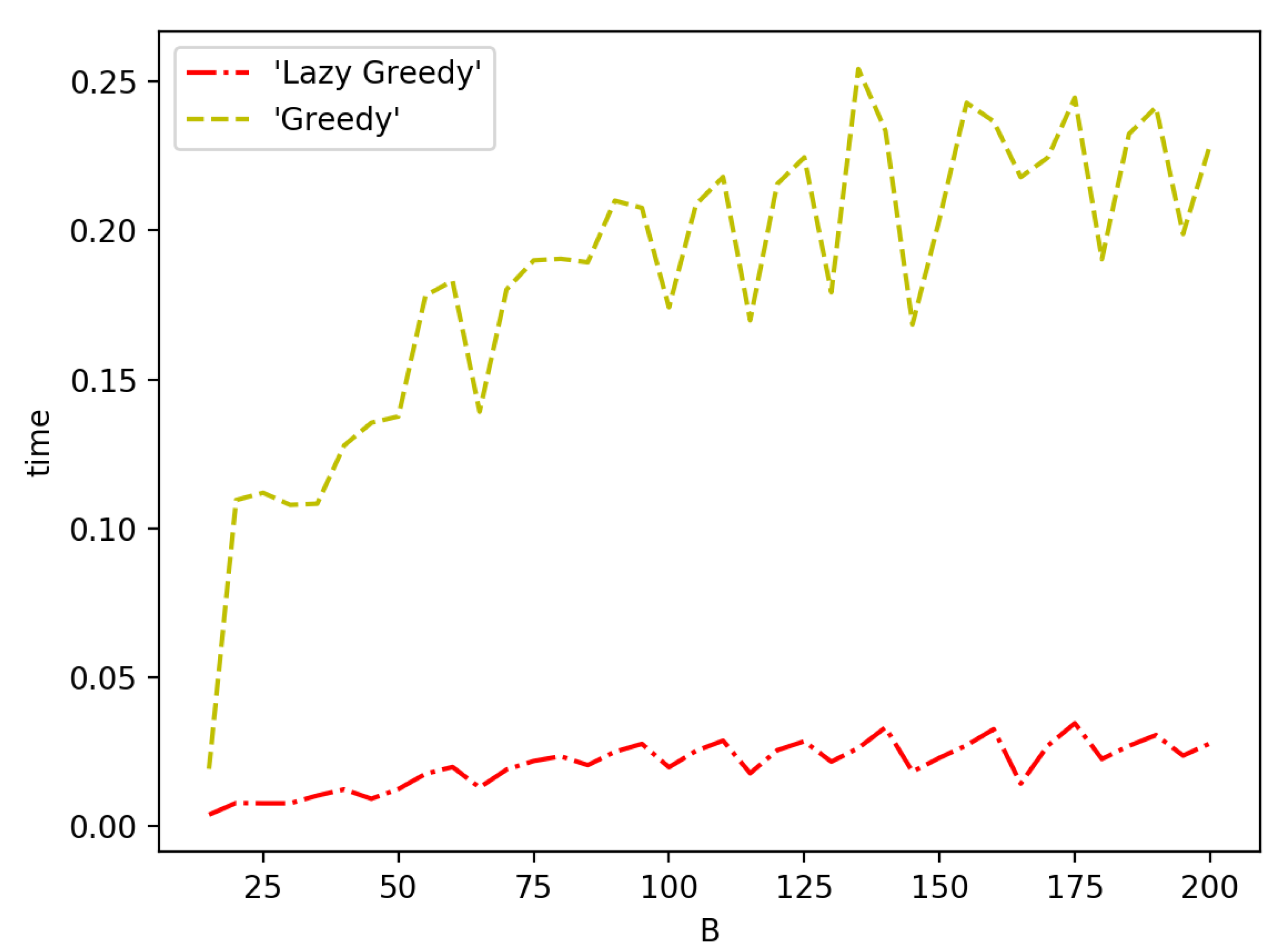
3.4. Speeding up the Algorithms
| Algorithm 3 Lazy greedy algorithm for one-with-all case |
|
| Algorithm 4 Lazy greedy algorithm for the general cost case |
|
4. Simulations
5. Conclusions
Author Contributions
Funding
Conflicts of Interest
References
- Sun, C.; Yu, Y.; Li, V.O.; Lam, J.C. Optimal Multi-type Sensor Placements in Gaussian Spatial Fields for Environmental Monitoring. In Proceedings of the 4th international conference on smart cities, Kansas City, MO, USA, 16–19 September 2018; pp. 420–429. [Google Scholar]
- Bacco, M.; Delmastro, F.; Ferro, E.; Gotta, A. Environmental Monitoring for Smart Cities. IEEE Sens. J. 2017, 17, 7767–7774. [Google Scholar] [CrossRef]
- Fischer, P.H.; Marra, M.; Ameling, C.B.; Hoek, G.; Beelen, R.; de Hoogh, K.; Breugelmans, O.; Kruize, H.; Janssen, N.A.; Houthuijs, D. Air pollution and mortality in seven million adults: The Dutch Environmental Longitudinal Study (DUELS). Environ. Health Perspect. 2015, 123, 697–704. [Google Scholar] [CrossRef] [PubMed]
- Kioumourtzoglou, M.A.; Schwartz, J.D.; Weisskopf, M.G.; Melly, S.J.; Wang, Y.; Dominici, F.; Zanobetti, A. Long-term PM2.5 exposure and neurological hospital admissions in the northeastern United States. Environ. Health Perspect. 2016, 124, 23–29. [Google Scholar] [CrossRef] [PubMed]
- Watts, N.; Adger, W.N.; Agnolucci, P.; Blackstock, J.; Byass, P.; Cai, W.; Chaytor, S.; Colbourn, T.; Collins, M.; Cooper, A.; et al. Health and climate change: Policy responses to protect public health. Lancet 2015, 386, 1861–1914. [Google Scholar] [CrossRef]
- Castell, N.; Dauge, F.R.; Schneider, P.; Vogt, M.; Lerner, U.; Fishbain, B.; Broday, D.; Bartonova, A. Can commercial low-cost sensor platforms contribute to air quality monitoring and exposure estimates? Environ. Int. 2017, 99, 293–302. [Google Scholar] [CrossRef] [PubMed]
- Beijing Air Pollution: Real-Time Air Quality Index (AQI). Available online: https://aqicn.org (accessed on 5 May 2018).
- Krause, A.; Singh, A.; Guestrin, C. Near-optimal sensor placements in Gaussian processes: Theory, efficient algorithms and empirical studies. J. Mach. Learn. Res. 2008, 9, 235–284. [Google Scholar]
- Leskovec, J.; Krause, A.; Guestrin, C.; Faloutsos, C.; VanBriesen, J.; Glance, N. Cost-effective outbreak detection in networks. In Proceedings of the 13th ACM SIGKDD International Conference on Knowledge Discovery and Data Mining, San Jose, CA, USA, 12–15 August 2007; pp. 420–429. [Google Scholar]
- Du, W.; Xing, Z.; Li, M.; He, B.; Chua, L.H.C.; Miao, H. Optimal sensor placement and measurement of wind for water quality studies in urban reservoirs. In Proceedings of the 13th International Symposium on Information Processing in Sensor Networks, Berlin, Germany, 15–17 April 2014; pp. 167–178. [Google Scholar]
- Wu, X.; Liu, M.; Wu, Y. In-situ soil moisture sensing: Optimal sensor placement and field estimation. ACM Trans. Sens. Netw. 2012, 8, 33. [Google Scholar] [CrossRef]
- Hsieh, H.P.; Lin, S.D.; Zheng, Y. Inferring air quality for station location recommendation based on urban big data. In Proceedings of the 21th ACM SIGKDD International Conference on Knowledge Discovery and Data Mining, Sydney, Australia, 10–13 August 2015; pp. 437–446. [Google Scholar]
- Singh, A.; Guillory, A.; Bilmes, J. On bisubmodular maximization. In Proceedings of the Artificial Intelligence and Statistics, Canary Islands, Spain, 21–23 April 2012; pp. 1055–1063. [Google Scholar]
- Ohsaka, N.; Yoshida, Y. Monotone k-submodular function maximization with size constraints. In Proceedings of the Advances in Neural Information Processing Systems, Montreal, QC, Canada, 7–12 December 2015; pp. 694–702. [Google Scholar]
- Array of Things: A Networked Urban Sensor Project in Chicago. Available online: https://arrayofthings.github.io/ (accessed on 5 May 2018).
- Hong Kong Air Quality Monitoring Data. Available online: http://www.aqhi.gov.hk/en.html (accessed on 5 May 2018).
- Yuen, K.V.; Kuok, S.C. Efficient Bayesian sensor placement algorithm for structural identification: A general approach for multi-type sensory systems. Earthq. Eng. Struct. Dyn. 2015, 44, 757–774. [Google Scholar] [CrossRef]
- Lin, J.F.; Xu, Y.L.; Law, S.S. Structural damage detection-oriented multi-type sensor placement with multi-objective optimization. J. Sound Vib. 2018, 422, 568–589. [Google Scholar] [CrossRef]
- Rasmussen, C.E. Gaussian processes in machine learning. In Advanced Lectures on Machine Learning; Springer: Berlin, Germany, 2004; pp. 63–71. [Google Scholar]
- Nott, D.J.; Dunsmuir, W.T. Estimation of nonstationary spatial covariance structure. Biometrika 2002, 89, 819–829. [Google Scholar] [CrossRef]
- Cressie, N. Statistics for Spatial Data; John Wiley & Sons: Hoboken, NJ, USA, 2015. [Google Scholar]
- Ko, C.W.; Lee, J.; Queyranne, M. An exact algorithm for maximum entropy sampling. Oper. Res. 1995, 43, 684–691. [Google Scholar] [CrossRef]
- Nemhauser, G.L.; Wolsey, L.A.; Fisher, M.L. An analysis of approximations for maximizing submodular set functions I. Math. Program. 1978, 14, 265–294. [Google Scholar] [CrossRef]
- Grant, M.; Boyd, S.; Ye, Y. CVX: Matlab Software for Disciplined Convex Programming. Available online: http://cvxr.com/cvx (accessed on 5 May 2018).
- Khuller, S.; Moss, A.; Naor, J.S. The budgeted maximum coverage problem. Inf. Process. Lett. 1999, 70, 39–45. [Google Scholar] [CrossRef]
- Sviridenko, M. A note on maximizing a submodular set function subject to a knapsack constraint. Oper. Res. Lett. 2004, 32, 41–43. [Google Scholar] [CrossRef]
- Air Pollution. Available online: https://www.who.int/sustainable-development/cities/health-risks/air-pollution/en/ (accessed on 5 May 2018).
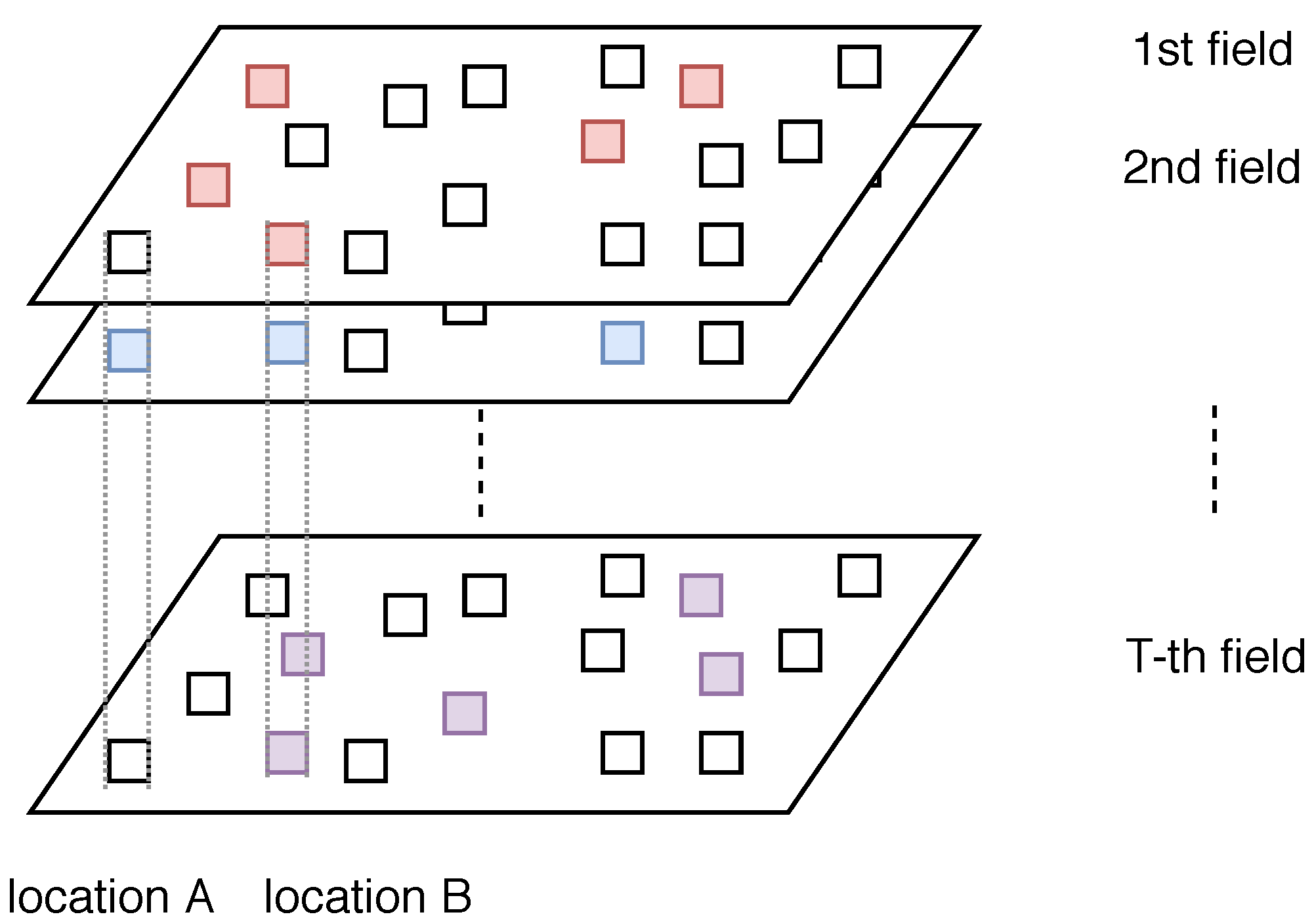
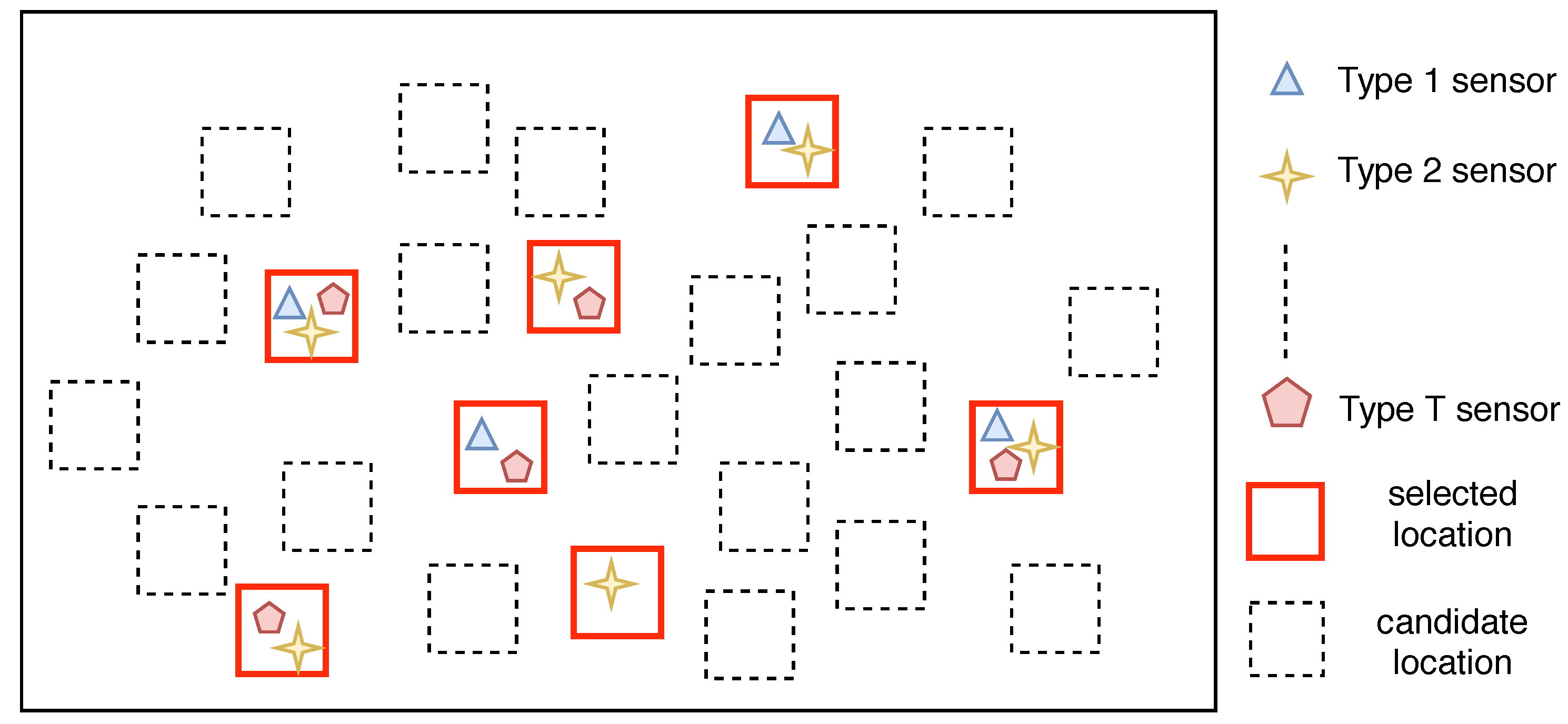
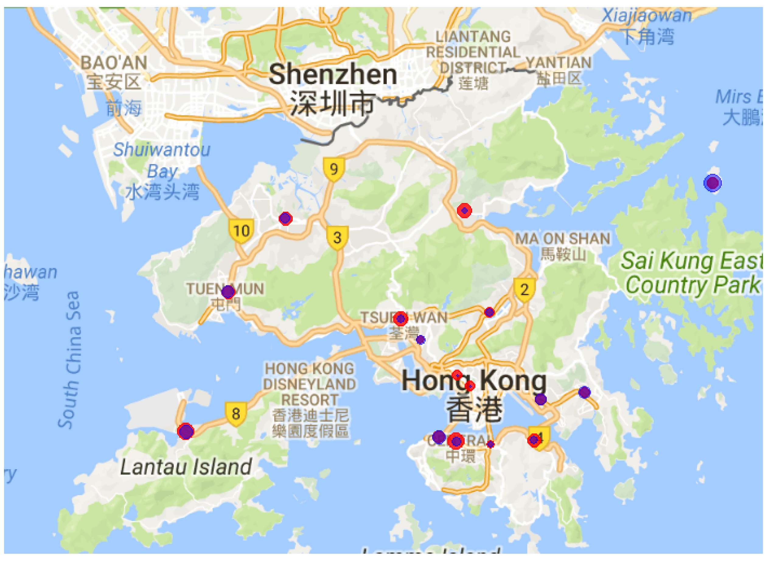


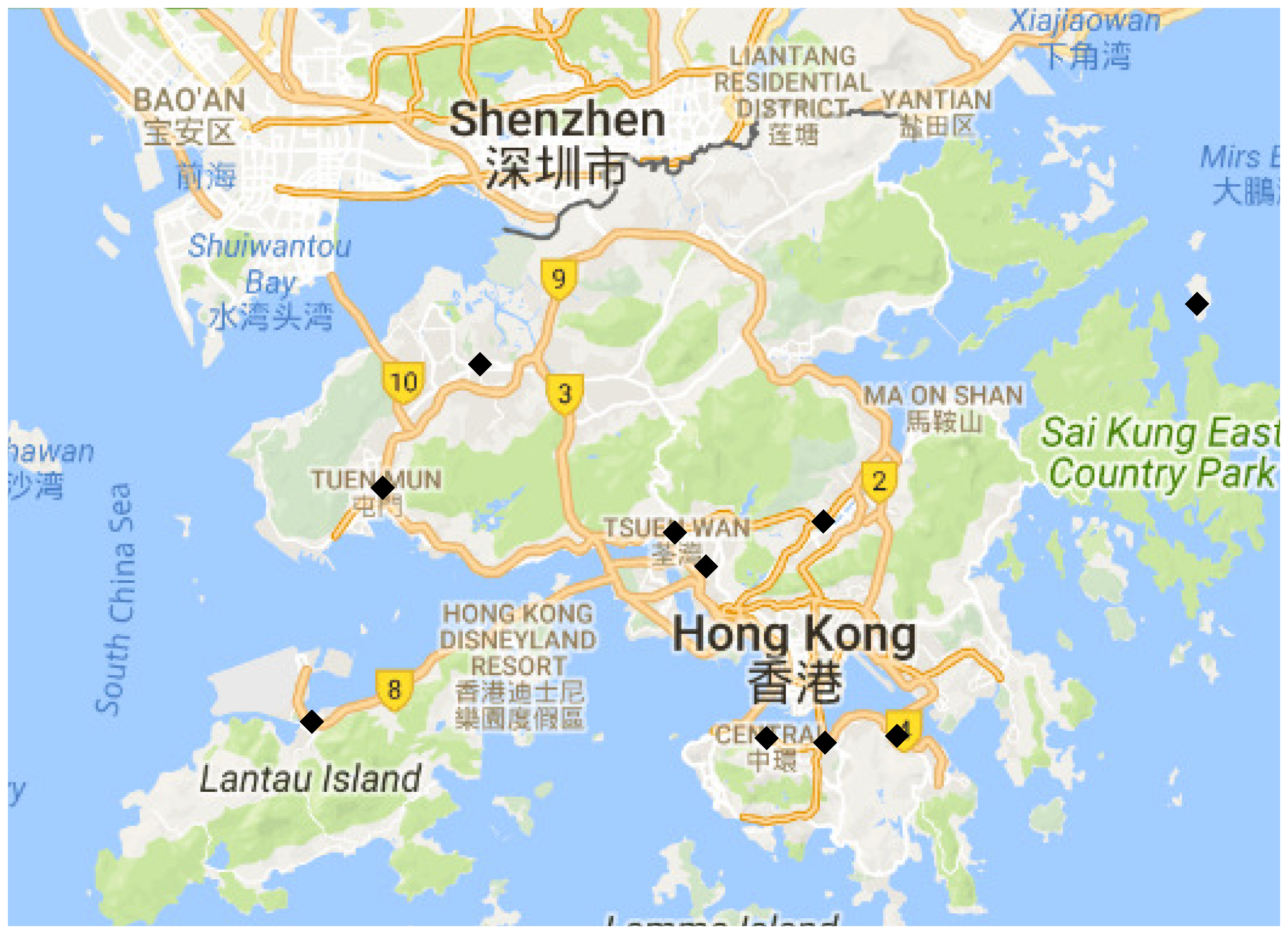
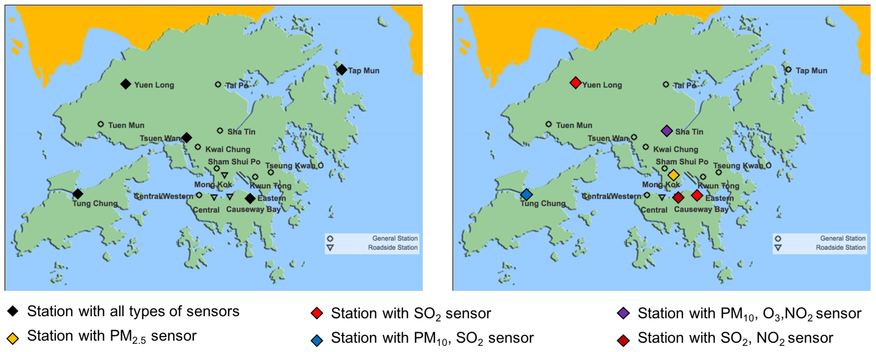
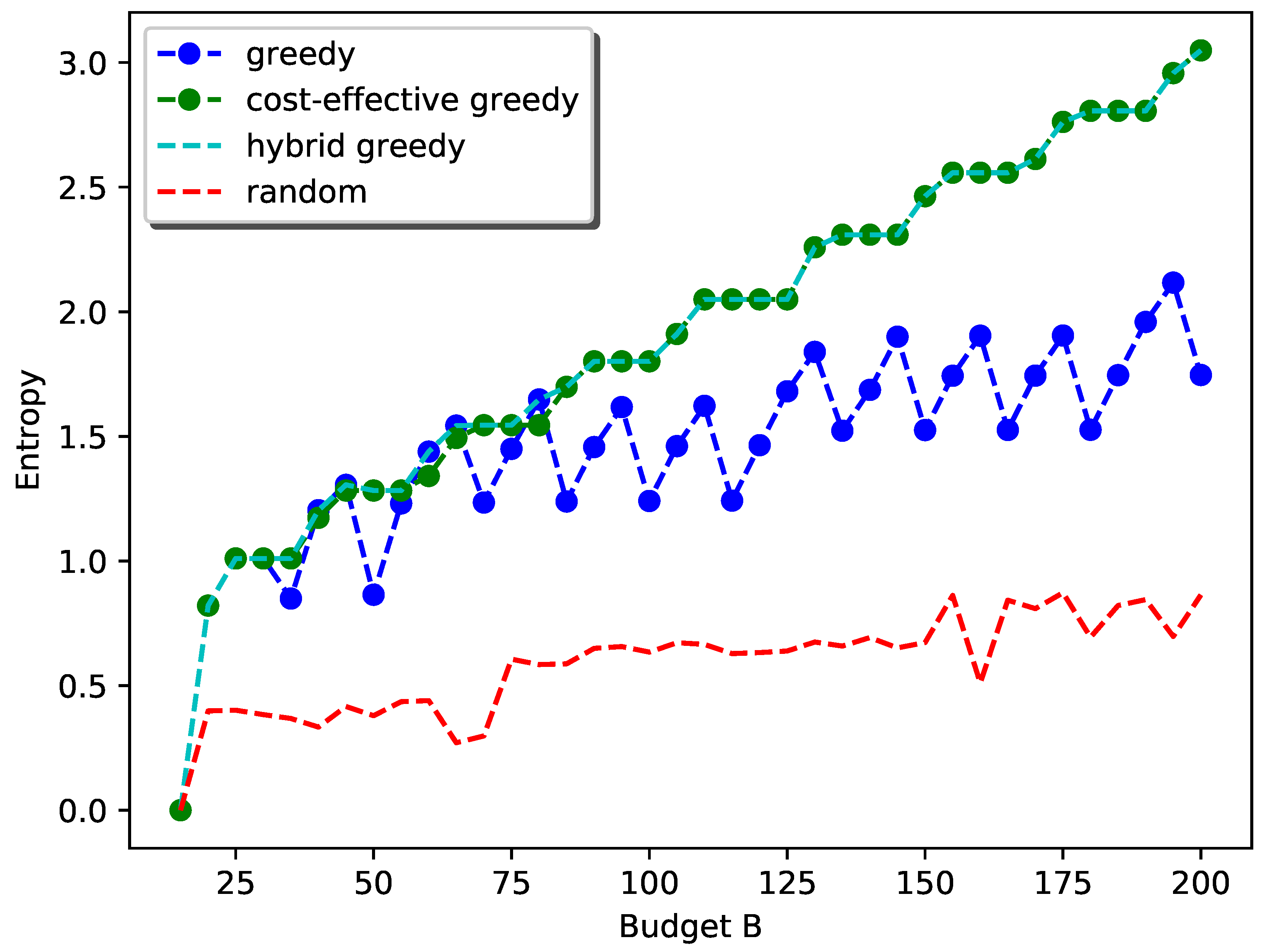
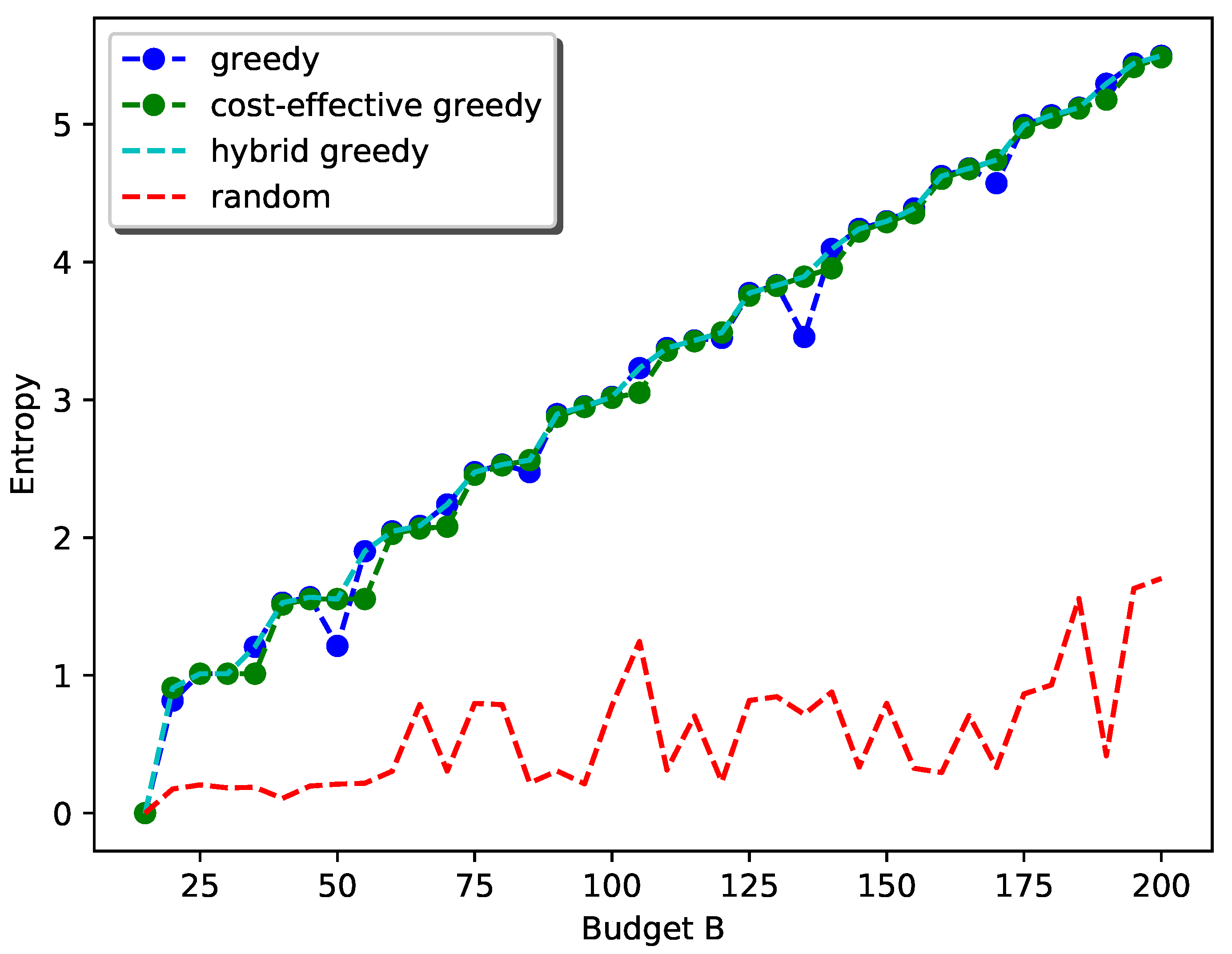
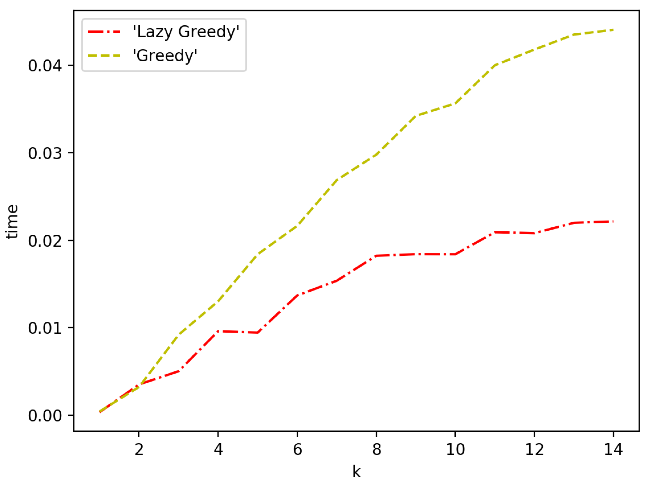
| Notation | Definition |
|---|---|
| The mean function of the Gaussian Process | |
| The kernel function of the Gaussian Process | |
| The random variables over the location index set A | |
| Try to span the whole column of the table | |
| T | The total number of types of interest |
| The abbreviation for the set | |
| V | The set of all indexes, each corresponding to a location/grid |
| The number of indexes in the set V | |
| s | an index in the set V |
| The set of the indexes of the selected locations for the ith type | |
| The placement scheme | |
| The ithe objective function | |
| The weight parameter of the ith objective function | |
| The unit cost for the ith type | |
| The site construction cost | |
| B | The total budget constraint |
| K | The subset size constraint |
| The total number of sensors for the ith type | |
| The floor function mapping x to the greatest integer | |
| less than or equal to x | |
| The information gain of adding location index s of type i |
© 2019 by the authors. Licensee MDPI, Basel, Switzerland. This article is an open access article distributed under the terms and conditions of the Creative Commons Attribution (CC BY) license (http://creativecommons.org/licenses/by/4.0/).
Share and Cite
Sun, C.; Yu, Y.; Li, V.O.K.; Lam, J.C.K. Multi-Type Sensor Placements in Gaussian Spatial Fields for Environmental Monitoring. Sensors 2019, 19, 189. https://doi.org/10.3390/s19010189
Sun C, Yu Y, Li VOK, Lam JCK. Multi-Type Sensor Placements in Gaussian Spatial Fields for Environmental Monitoring. Sensors. 2019; 19(1):189. https://doi.org/10.3390/s19010189
Chicago/Turabian StyleSun, Chenxi, Yangwen Yu, Victor O. K. Li, and Jacqueline C. K. Lam. 2019. "Multi-Type Sensor Placements in Gaussian Spatial Fields for Environmental Monitoring" Sensors 19, no. 1: 189. https://doi.org/10.3390/s19010189
APA StyleSun, C., Yu, Y., Li, V. O. K., & Lam, J. C. K. (2019). Multi-Type Sensor Placements in Gaussian Spatial Fields for Environmental Monitoring. Sensors, 19(1), 189. https://doi.org/10.3390/s19010189


