Semi-Supervised Segmentation Framework Based on Spot-Divergence Supervoxelization of Multi-Sensor Fusion Data for Autonomous Forest Machine Applications


 ,
,
Abstract
1. Introduction
2. Related Works
2.1. Point Clouds-Based Segmentation Method
2.2. Supervoxel Process
2.3. Supervoxel-Based Segmentation Method
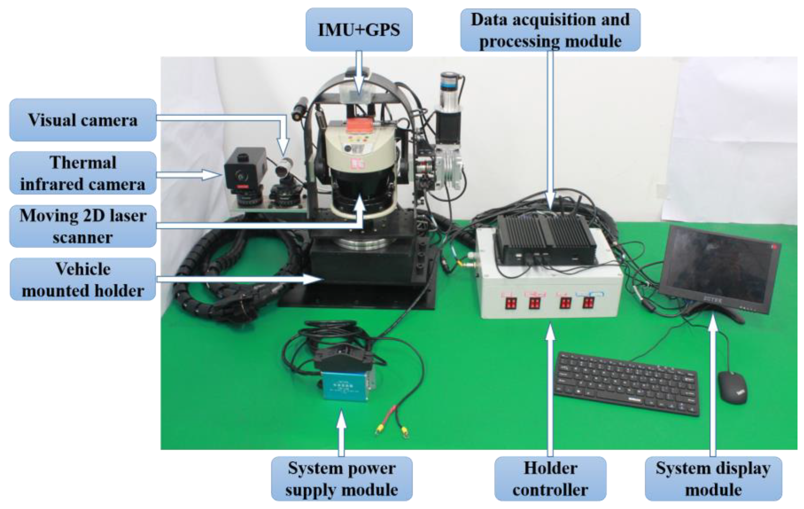
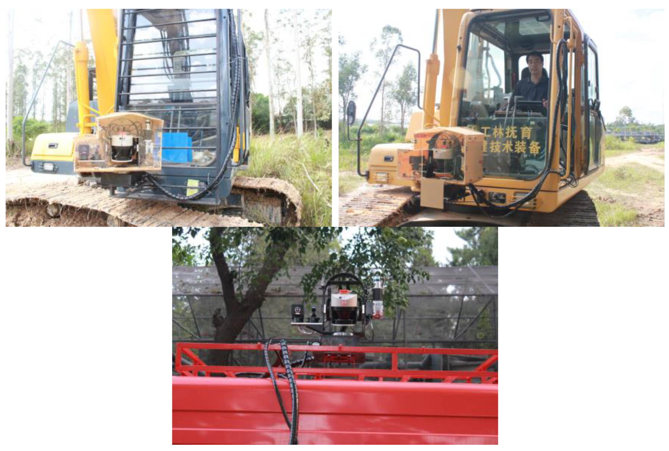
3. Multi-Sensor Measuring System
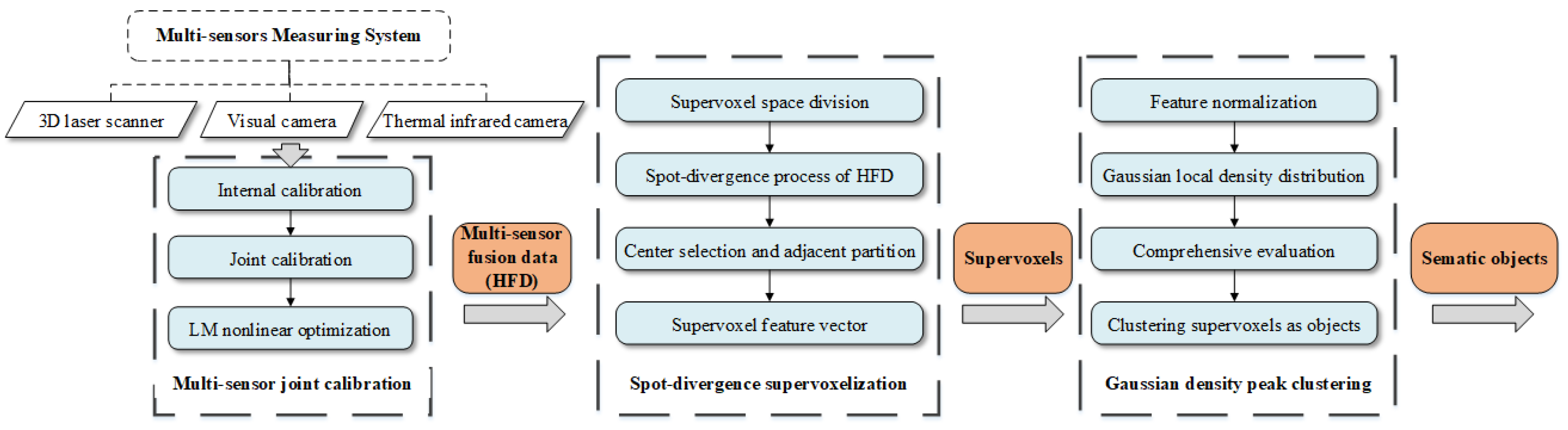
4. Methodology
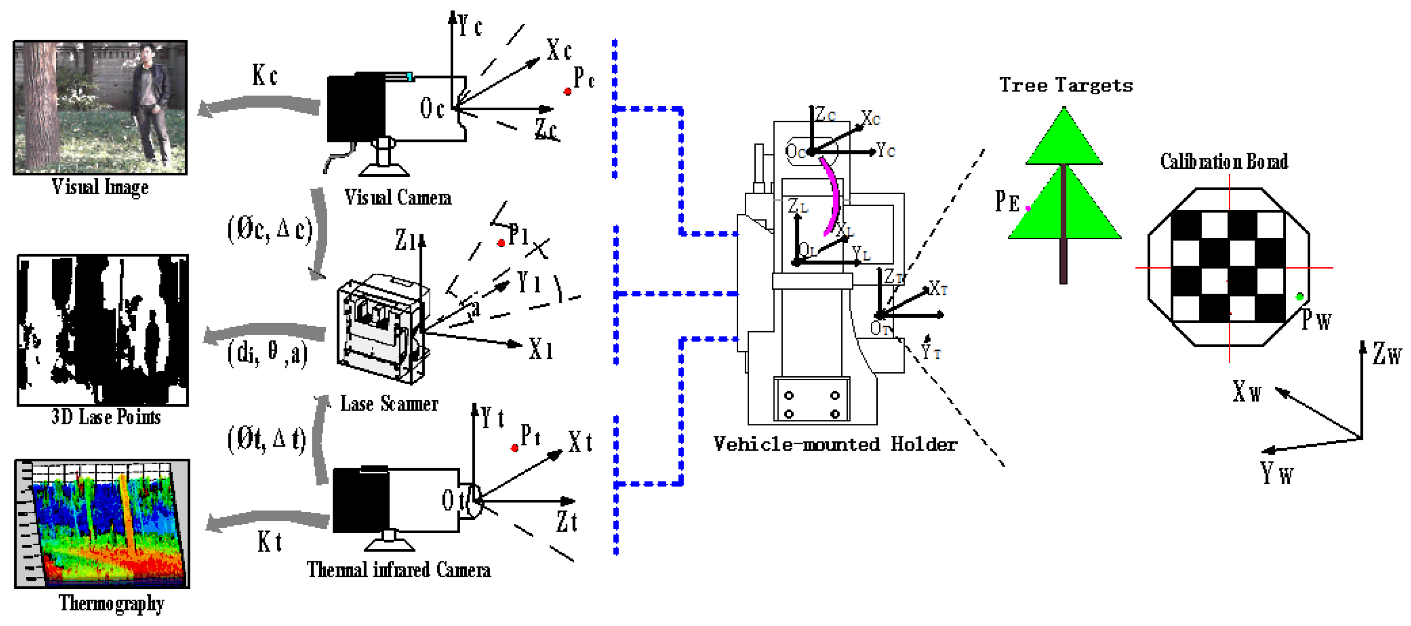
4.1. Multi-Sensor Joint Calibration
4.2. Spot-Divergence Supervoxelization
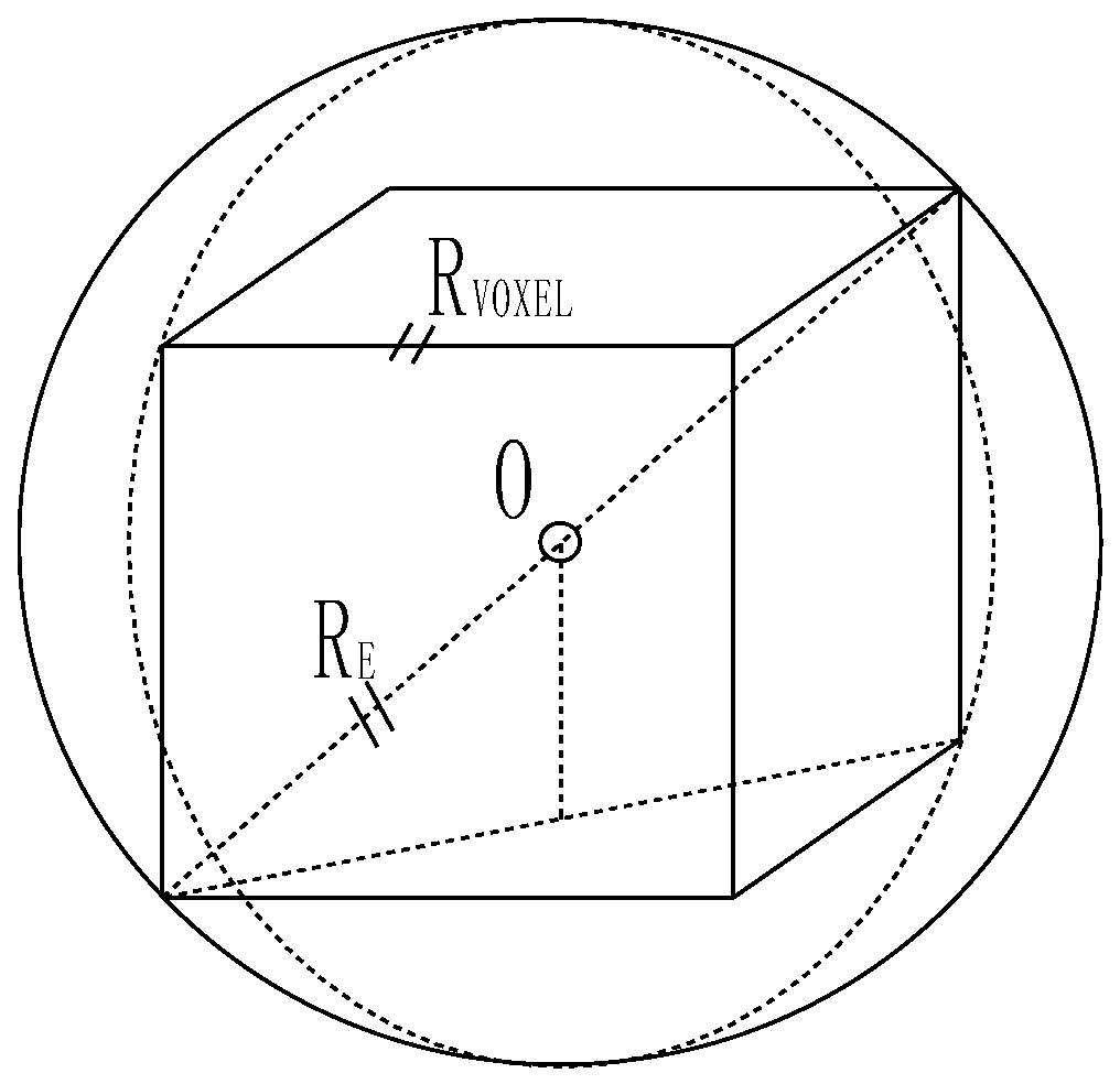
4.2.1. Supervoxel Space Division
4.2.2. Spot-Divergence Process of HFD
4.2.3. Center Selection and Adjacent Partition
4.2.4. Supervoxel Feature Vector
- 1)
- Spatial coordinates of supervoxel center:
- 2)
- CIELAB color average of n HFD in the supervoxel:
- 3)
- Temperature average of the supervoxel:
- 4)
- Reflectance average of the supervoxel:
- 5)
- Edge length mean of n HFD in the supervoxel:
- 6)
- Absolute range between maximum and minimum of :
- 7)
- Surface normal vector of supervoxel: with
- 8)
- Comprehensive dissimilarity of vectors:
4.3. Gaussian Density Peak Clustering
4.3.1. Feature Normalization
4.3.2. Gaussian Local Density Distribution
4.3.3. Clustering Supervoxels as Objects
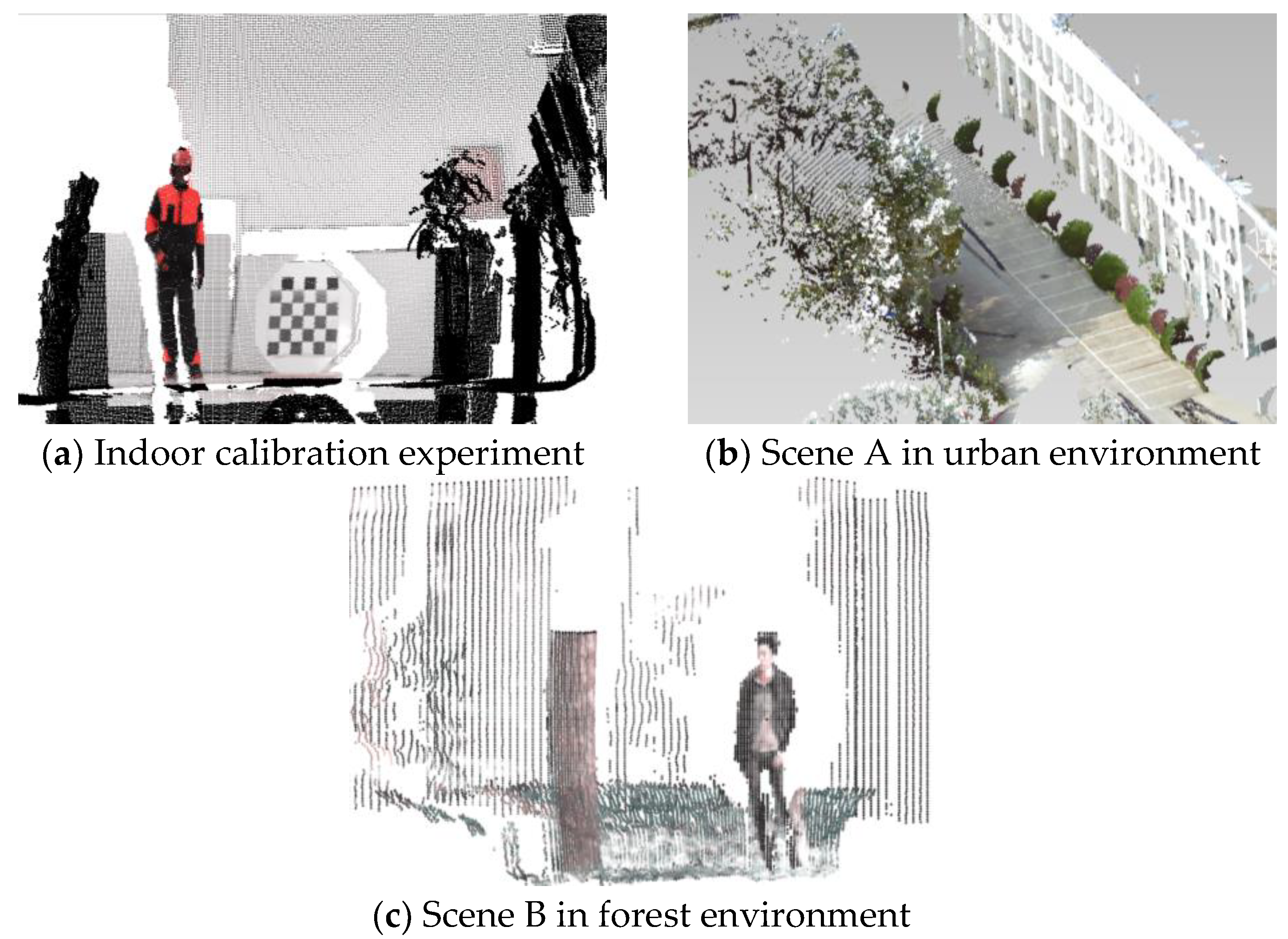
5. Results and Analysis
5.1. Multi-Sensor Fusion Evaluation
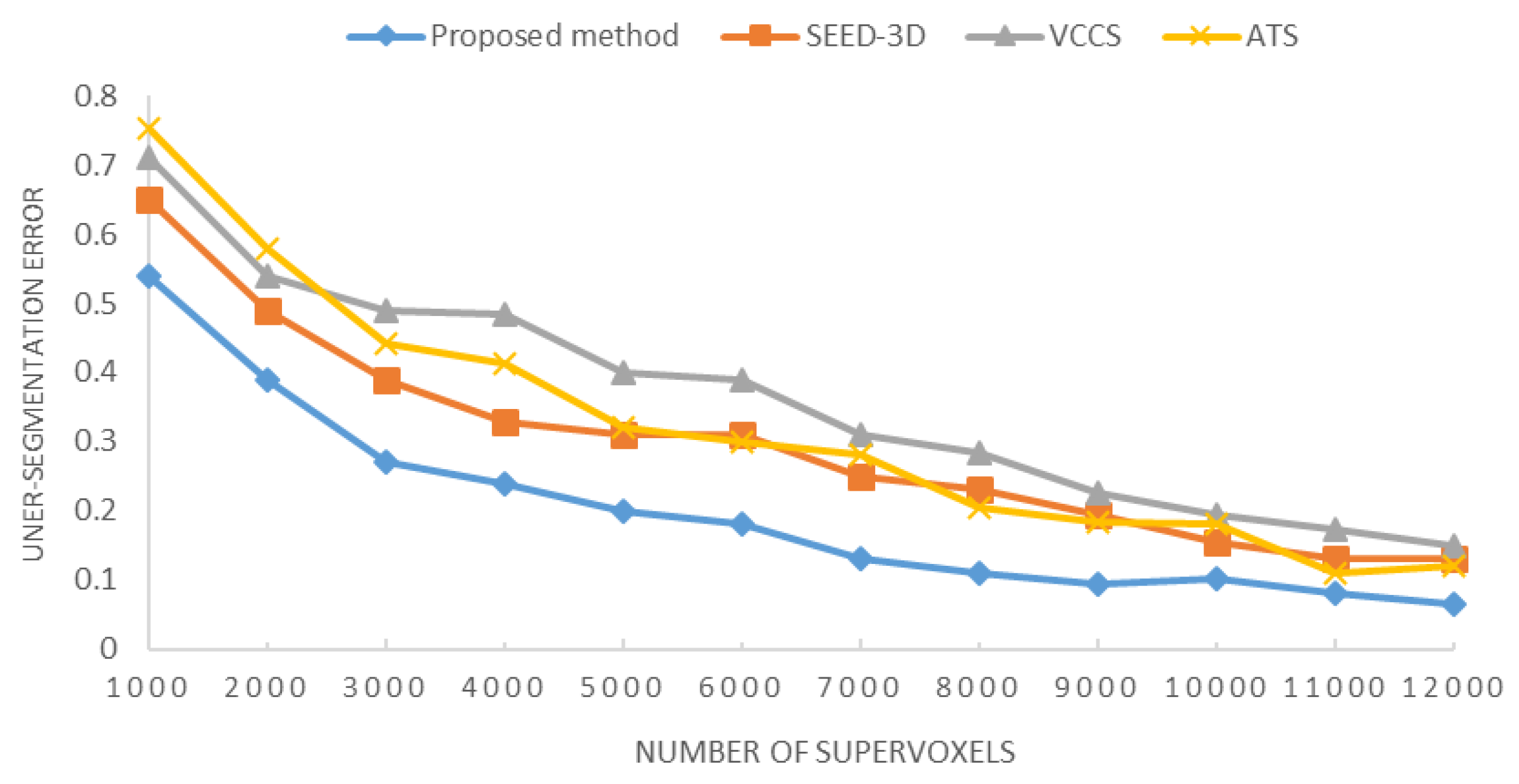
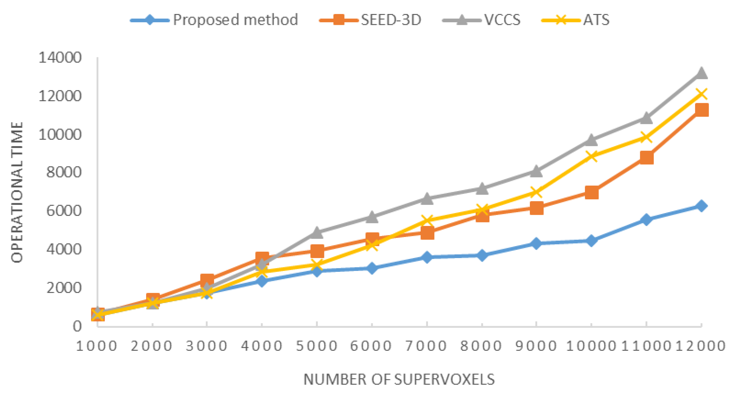
5.2. Supervoxelization Evaluation
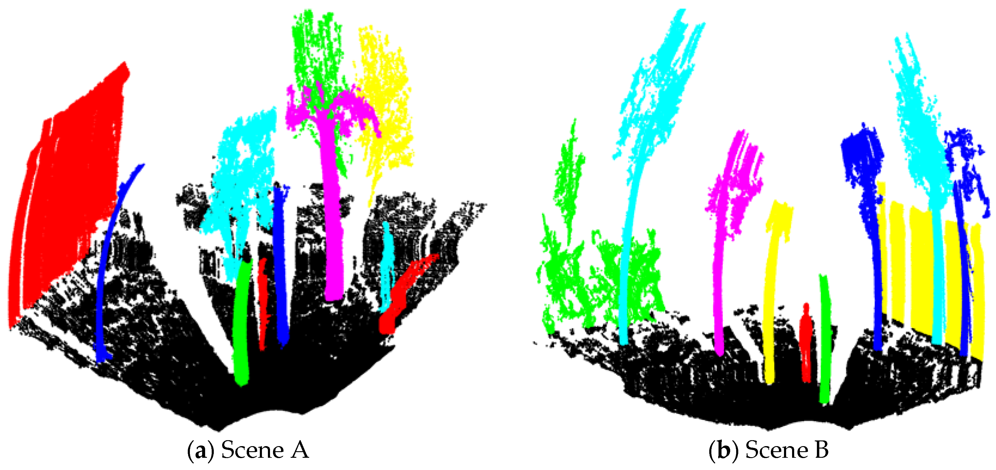
5.3. Semantic Segmentation Evaluation
6. Conclusions
Author Contributions
Funding
Conflicts of Interest
References
- Waser, L.T.; Boesch, R.; Wang, Z.; Ginzler, C. Towards Automated Forest Mapping. In Mapping Forest Landscape Patterns; Springer: New York, NY, USA, 2017. [Google Scholar]
- Qian, C.; Liu, H.; Tang, J.; Chen, Y.; Kaartinen, H.; Kukko, A.; Zhu, L.; Liang, X.; Chen, L.; Hyyppä, J. An Integrated GNSS/INS/LiDAR-SLAM Positioning Method for Highly Accurate Forest Stem Mapping. Remote. Sens. 2016, 9, 3. [Google Scholar] [CrossRef]
- Becker, R.; Keefe, R.; Anderson, N. Use of Real-Time GNSS-RF Data to Characterize the Swing Movements of Forestry Equipment. Forests 2017, 8, 44. [Google Scholar] [CrossRef]
- Heinzel, J.; Huber, M.O. Detecting Tree Stems from Volumetric TLS Data in Forest Environments with Rich Understory. Remote. Sens. 2016, 9, 9. [Google Scholar] [CrossRef]
- Kong, J.L.; Ding, X.K.; Liu, J.; Yan, L.; Wang, J. New Hybrid Algorithms for Estimating Tree Stem Diameters at Breast Height Using a Two Dimensional Terrestrial Laser Scanner. Sensors 2015, 15, 15661–15683. [Google Scholar] [CrossRef] [PubMed]
- Thomas, H.; Pär, L.; Tomas, N.; Ola, R. Autonomous Forest Vehicles: Historic, envisioned, and state-of-the-art. J. For. Eng. 2009, 20, 31–38. [Google Scholar]
- Miettinen, M.; Ohman, M.; Visala, A.; Forsman, P. Simultaneous Localization and Mapping for Forest Harvesters. In Proceedings of the IEEE International Conference on Robotics and Automation, Roma, Italy, 10–14 April 2007; pp. 517–522. [Google Scholar]
- Engelmann, F.; Kontogianni, T.; Hermans, A.; Leibe, B. Exploring Spatial Context for 3D Semantic Segmentation of Point Clouds. In Proceedings of the IEEE International Conference on Computer Vision Workshop, Venice, Italy, 22–29 October 2017; pp. 716–724. [Google Scholar]
- Marinello, F.; Proto, A.R.; Zimbalatti, G.; Pezzuolo, A.; Cavalli, R.; Grigolato, S. Determination of forest road surface roughness by Kinect depth imaging. Ann. For. Res. 2017, 60. [Google Scholar] [CrossRef]
- Giusti, A.; Guzzi, J.; Dan, C.C.; He, F.-L.; Rodriguez, J.P.; Fontana, F.; Faessler, M.; Forster, C.; Schmidhuber, J.; Caro, G.D.; et al. A Machine Learning Approach to Visual Perception of Forest Trails for Mobile Robots. IEEE Robot. Autom. Lett. 2017, 1, 661–667. [Google Scholar] [CrossRef]
- Xu, Y.; Tuttas, S.; Hoegner, L.; Stilla, U. Voxel-based segmentation of 3D point clouds from construction sites using a probabilistic connectivity model. Pattern Recognit. Lett. 2018, 102, 67–74. [Google Scholar] [CrossRef]
- Trochta, J.; Krůček, M.; Vrška, T.; Král, K. 3D Forest: An application for descriptions of three-dimensional forest structures using terrestrial LiDAR. PLoS ONE 2017, 12, e0176871. [Google Scholar] [CrossRef] [PubMed]
- Ramiya, A.M.; Nidamanuri, R.R.; Krishnan, R. Segmentation based building detection approach from LiDAR point cloud. Egypt. J. Remote. Sens. Space Sci. 2016, 20, 71–77. [Google Scholar] [CrossRef]
- Yang, B.; Dai, W.; Dong, Z.; Liu, Y. Automatic Forest Mapping at Individual Tree Levels from Terrestrial Laser Scanning Point Clouds with a Hierarchical Minimum Cut Method. Remote. Sens. 2016, 8, 372. [Google Scholar] [CrossRef]
- Hamraz, H.; Contreras, M.A.; Zhang, J. Forest understory trees can be segmented accurately within sufficiently dense airborne laser scanning point clouds. Sci. Rep. 2017, 7, 6770. [Google Scholar] [CrossRef] [PubMed]
- Vo, A.V.; Truong-Hong, L.; Laefer, D.F.; Bertolotto, M. Octree-based region growing for point cloud segmentation. ISPRS J. Photogramm. Remote. Sens. 2015, 104, 88–100. [Google Scholar] [CrossRef]
- Zhong, L.; Cheng, L.; Xu, H.; Wu, Y.; Chen, Y.; Li, M. Segmentation of Individual Trees from TLS and MLS Data. IEEE J. Sel. Top. Appl. Earth Obs. Remote Sens. 2017, 10, 774–787. [Google Scholar] [CrossRef]
- Weinmann, M.; Weinmann, M.; Mallet, C.; Brédif, M. A Classification-Segmentation Framework for the Detection of Individual Trees in Dense MMS Point Cloud Data Acquired in Urban Areas. Remote Sens. 2017, 9, 277. [Google Scholar] [CrossRef]
- Achanta, R.; Shaji, A.; Lucchi, A.; Lucchi, A.; Fua, P.; Süsstrunk, S. SLIC superpixels compared to state-of-the-art superpixel methods. IEEE Trans. Pattern Anal. Mach. Intell. 2012, 34, 2274–2282. [Google Scholar] [CrossRef] [PubMed]
- Van, D.; Bergh, M.; Boix, X.; Roig, G.; Van Gool, L. SEEDS: Superpixels extracted via energy-driven sampling. Int. J. Comput. Vis. 2015, 111, 298–314. [Google Scholar]
- Papon, J.; Abramov, A.; Schoeler, M.; Worgotter, F. Voxel Cloud Connectivity Segmentation—Supervoxels for Point Clouds. In Proceedings of the IEEE Conference on Computer Vision Pattern Recognition, Portland, OR, USA, 23–28 June 2013; pp. 2027–2034. [Google Scholar]
- Kim, J.S.; Park, J.H. Weighted-graph-based supervoxel segmentation of 3D point clouds in complex urban environment. Electron. Lett. 2015, 51, 1789–1791. [Google Scholar] [CrossRef]
- Ban, Z.; Chen, Z.; Liu, J. Supervoxel Segmentation with Voxel-Related Gaussian Mixture Model. Sensors 2018, 18, 128. [Google Scholar]
- Xu, S.; Ye, N.; Xu, S.; Zhu, F. A supervoxel approach to the segmentation of individual trees from LiDAR point clouds. Remote Sens. Lett. 2018, 9, 515–523. [Google Scholar] [CrossRef]
- Aijazi, A.K.; Checchin, P.; Trassoudaine, L. Segmentation Based Classification of 3D Urban Point Clouds: A Super-Voxel Based Approach with Evaluation. Remote Sens. 2013, 5, 1624–1650. [Google Scholar] [CrossRef]
- Li, M.; Sun, C. Refinement of LiDAR point clouds using a super voxel based approach. J. Photogramm. Remote. Sens. 2018. [Google Scholar] [CrossRef]
- Yun, J.S.; Sim, J.Y. Supervoxel-based saliency detection for large-scale colored 3D point clouds. In Proceedings of the IEEE International Conference on Image Processing, Phoenix, AZ, USA, 25–28 September 2016; pp. 4062–4066. [Google Scholar]
- Verdoja, F.; Thomas, D.; Sugimoto, A. Fast 3D point cloud segmentation using supervoxels with geometry and color for 3D scene understanding. In Proceedings of the 2017 IEEE International Conference on Multimedia and Expo (ICME), Hong Kong, China, 10–14 July 2017; pp. 1285–1290. [Google Scholar]
- Wu, F.; Wen, C.; Guo, Y.; Wang, J.; Yu, Y.; Wang, C.; Li, J. Rapid Localization and Extraction of Street Light Poles in Mobile LiDAR Point Clouds: A Supervoxel-Based Approach. IEEE Trans. Intell. Transp. Syst. 2017, 18, 292–305. [Google Scholar] [CrossRef]
- Alex, R.; Alessandro, L. Machine learning. Clustering by fast search and find of density peaks. Science 2014, 344, 1492–1496. [Google Scholar]
- Wang, S.; Wang, D.; Caoyuan, L.I.; Li, Y. Clustering by Fast Search and Find of Density Peaks with Data Field. Chin. J. Electron. 2017, 25, 397–402. [Google Scholar] [CrossRef]
- Zhang, Z. A Flexible New Technique for Camera Calibration. IEEE Trans. Pattern Anal. Mach. Intell. 2000, 22, 1330–1334. [Google Scholar] [CrossRef]
- Kong, J.; Li, F.; Liu, J.; Yan, L.; Ding, X. New Calibration Method of Two-Dimensional Laser Scanner and Camera Based on LM-BP Neural Network. Int. J. Signal Process. Image Process. Pattern Recognit. 2016, 9, 231–244. [Google Scholar] [CrossRef]
- Lourakis, M.I.A. A Brief Description of the Levenberg-Marquardt Algorithm Implemened by Levmar; Foundation of Research & Technology: Heraklion, Greece, 2005. [Google Scholar]
- SICK Sensor Intelligence, Operating Instructions: Laser Measurement Sensors of the LMS5xx Product Family. SICK AG Waldkirch, 2012. Available online: https://www.sick.com/cn/zh/ (accessed on 11 September 2018).
- Rusu, R.B.; Cousins, S. 3D is here: Point Cloud Library (PCL). In Proceedings of the IEEE International Conference on Robotics and Automation, Shanghai, China, 9–13 May 2011. [Google Scholar]


| Parameters | Calibration Work in [33] | Proposed Calibration Work |
|---|---|---|
| Average calibration offset error | 5.819 (cm) | 2.764 (cm) |
| Average angular error | 1.164° | 0.553° |
| RMSE | 8.232 | 5.126 |
| STD | 19.823 | 13.032 |
| Ground | Pedestrian | Tree | Shrub | Building | Stone | Average | |
|---|---|---|---|---|---|---|---|
| Ground | 14048 | 12 | 17 | 63 | 76 | 24 | |
| Pedestrian | 6 | 410 | 5 | 1 | 0 | 11 | |
| Tree | 13 | 2 | 2208 | 65 | 3 | 5 | |
| Shrub | 19 | 4 | 35 | 1526 | 13 | 6 | |
| Building | 26 | 0 | 9 | 12 | 2672 | 15 | |
| Stone | 15 | 16 | 0 | 4 | 9 | 492 | |
| Precision | 0.987 | 0.947 | 0.962 | 0.952 | 0.977 | 0.918 | 0.957 |
| Recall | 0.994 | 0.923 | 0.971 | 0.913 | 0.964 | 0.890 | 0.943 |
| F value | 0.990 | 0.935 | 0.966 | 0.932 | 0.970 | 0.904 | 0.950 |
| Ground | Pedestrian | Tree | Shrub | Building | Average | |
|---|---|---|---|---|---|---|
| Ground | 8145 | 24 | 26 | 149 | 13 | |
| Pedestrian | 32 | 710 | 4 | 19 | 1 | |
| Tree | 66 | 7 | 5341 | 65 | 6 | |
| Shrub | 19 | 4 | 35 | 3476 | 1 | |
| Building | 44 | 11 | 29 | 12 | 832 | |
| Precision | 0.975 | 0.927 | 0.974 | 0.983 | 0.897 | 0.951 |
| Recall | 0.981 | 0.939 | 0.983 | 0.934 | 0.975 | 0.962 |
| F value | 0.978 | 0.933 | 0.978 | 0.958 | 0.934 | 0.956 |
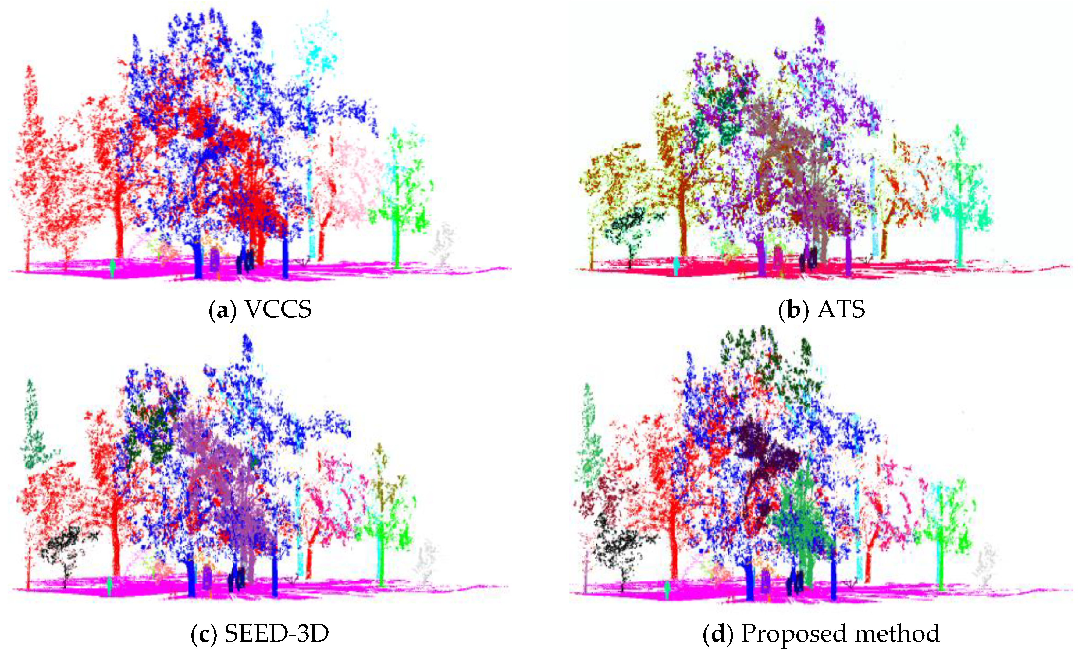
| Segmentation Algorithm | Integrated Clusters | Discrete Clusters | F Value | Time (Approximate) | Effective HDF |
|---|---|---|---|---|---|
| VCCS [21] + K-mean | 39 | 317 | 0.893 | 92 min | 803,252 |
| SEED-3D [22] + K-mean | 45 | 382 | 0.938 | 51 min | 756,328 |
| ATS [24] + K-mean | 48 | 426 | 0.920 | 65 min | 983,174 |
| Proposed method | 44 | 125 | 0.942 | 34 min | 1,139,829 |
© 2018 by the authors. Licensee MDPI, Basel, Switzerland. This article is an open access article distributed under the terms and conditions of the Creative Commons Attribution (CC BY) license (http://creativecommons.org/licenses/by/4.0/).
Share and Cite
Kong, J.-l.; Wang, Z.-n.; Jin, X.-b.; Wang, X.-y.; Su, T.-l.; Wang, J.-l. Semi-Supervised Segmentation Framework Based on Spot-Divergence Supervoxelization of Multi-Sensor Fusion Data for Autonomous Forest Machine Applications. Sensors 2018, 18, 3061. https://doi.org/10.3390/s18093061
Kong J-l, Wang Z-n, Jin X-b, Wang X-y, Su T-l, Wang J-l. Semi-Supervised Segmentation Framework Based on Spot-Divergence Supervoxelization of Multi-Sensor Fusion Data for Autonomous Forest Machine Applications. Sensors. 2018; 18(9):3061. https://doi.org/10.3390/s18093061
Chicago/Turabian StyleKong, Jian-lei, Zhen-ni Wang, Xue-bo Jin, Xiao-yi Wang, Ting-li Su, and Jian-li Wang. 2018. "Semi-Supervised Segmentation Framework Based on Spot-Divergence Supervoxelization of Multi-Sensor Fusion Data for Autonomous Forest Machine Applications" Sensors 18, no. 9: 3061. https://doi.org/10.3390/s18093061
APA StyleKong, J.-l., Wang, Z.-n., Jin, X.-b., Wang, X.-y., Su, T.-l., & Wang, J.-l. (2018). Semi-Supervised Segmentation Framework Based on Spot-Divergence Supervoxelization of Multi-Sensor Fusion Data for Autonomous Forest Machine Applications. Sensors, 18(9), 3061. https://doi.org/10.3390/s18093061