1. Introduction
The joint estimation of the Doppler and time delay of a noise-contaminated signal is a fundamental problem in radar and sonar systems and this has been extensively addressed for the case involving narrowband signals [
1,
2,
3,
4,
5,
6]. Weiss [
7], Remley [
8], and Qu [
9] indicated that the narrowband model and the corresponding narrowband signal processing techniques are applicable when
, where
is the bandwidth of the transmitted signal,
is the duration of the transmitted signal,
is the relative velocity between the target and the sensor, and
is the propagation speed of the signal. The wideband signals, such as linear frequency modulation (LFM) signals with a large time frequency–bandwidth product, are frequently used in sonar and radar systems because of their lower probability of interception. In many modern radar systems, however, a wideband signal is utilized, and the narrowband model is not appropriate. In applications where
is invalid, the wideband model has to be employed. In wideband radar systems, the echo often contains a Doppler stretch (DS), and not a Doppler shift only, which results in difficulty in the parameters’ estimation. For the determination of the range and the relative velocity of the target, the accurate estimation of these parameters is crucial.
Since the fractional Fourier transform (FRFT) spectrum of a LFM signal has a greater energy concentration characteristic, the FRFT, as a new time–frequency tool, has attracted more attention, and has been widely applied to the parameter estimation of LFM signal [
10,
11,
12,
13,
14,
15,
16]. Zhao et al. propose a method for estimating the LFM signal by utilizing the pulse compression in both the time domain and the FRFT domain [
10]. The parameters of the LFM signal can be estimated by a fractional Fourier transform [
11,
12], a fractional correlation [
13], and a fractional power spectrum [
14,
15,
16].
Up to now, in most parameter estimation methods for array signal processing, the additive noise is assumed to be Gaussian. Studies and experimental measurements have shown that a broad class of noise such as underwater acoustic noise, atmospheric noise, multiuser interference, and radar clutters in real world applications are non-Gaussian, primarily owing to impulsive phenomena [
17,
18]. Taking these scenarios into account, it is inappropriate to model the noise as Gaussian noise. Researchers have studied this impulsive nature, and shown that the symmetric alpha stable (
) processes are better models for impulsive noise than the Gaussian processes. The conventional algorithms based on second-order statistics degenerate severely in the
noise environment.
To reduce the
noise interference, many parameter estimation algorithms based on the fractional lower-order statistics (FLOS) have been proposed [
16,
19,
20,
21]. However, these algorithms do need a priori knowledge of the
noise and have other limitations, where the characteristic exponent
and the fractional lower order of moments
must meet the need of
or
, otherwise those algorithms performance can degrade seriously, or even become invalid, while the fractional lower-order moment value is not appropriate.
The Sigmoid function is widely used as a common nonlinear transform. The Sigmoid function can suppress impulsive noise interference, and this does not depend on a priori knowledge of the noise. Yu et al., propose a method based on generalized Sigmoid cyclic cross-ambiguity function to estimate the time delay and Doppler frequency shift in the impulsive noise and co-channel interference [
22]. In [
22], the signal is assumed to be the real signal. However, when the signal is a complex signal, the results do not always hold.
To handle this problem, a novel concept termed the tuneable Sigmoid transform fractional correlation (TS-FC) is proposed in this paper, and a relative method named the tuneable Sigmoid fractional power spectrum density (TS-FPSD) is presented, to fulfill the needs mentioned above. The novel algorithm based on the TS-FPSD is then proposed to estimate the Doppler stretch and time delay. In addition, we address unbiasedness and consistency by adding their corresponding derivation. Furthermore, the boundness of the TS-FPSD to the noise, the parameter selection of the TS-FPSD, the feasibility analysis of the TS-FPSD, and the Cramér–Rao bound for parameter estimation are presented, to evaluate the performance of the proposed method. The proposed method does not need a priori knowledge of the alpha stable distribution noise.
This paper is organized as follows.
Section 2 presents a signal model of wideband echoes in an alpha-stable distribution noise environment. In
Section 3, the analysis of the fractional power spectrum density is presented. In
Section 4, a novel tuneable Sigmoid fractional correlation function (TS-FC) and a novel tuneable Sigmoid fractional power spectrum density function (TS-FPSD) are defined. In addition, unbiasedness and consistency are derived. In
Section 5, a novel Doppler stretch and time delay estimation method based on TS-FPSD for the
noise is proposed. In addition, the boundness of the TS-FPSD to the
noise, parameter selection of the TS-FPSD, and a feasibility analysis of the TS-FPSD are analyzed, and the Cramér–Rao bound for parameter estimation is derived. In
Section 6, the performance of the parameter estimation algorithm is studied through extensive numerical simulations. Finally, conclusions are drawn in
Section 7.
5. Parameter Estimation Based on TS-FPSD
5.1. Joint Doppler Stretch and Time Delay Estimation
The echo signal
with
-stable distribution noise can be expressed as:
where the noise
denotes the
noise.
According to the definition of the TS-FC, the TS-FC
of the echo signal
can be expressed as:
According to the definition of the TS-FPSD, the TS-FPSD
of the signal
can be expressed as
The joint estimation method for the Doppler stretch
and the time delay
based on the TS-FPSD, is given by [
16]:
Accordingly, the estimation of the Doppler stretch and the time delay in wideband echoes for a LFM pulse radar under an alpha-stable distribution noise was achieved via the proposed tuneable Sigmoid fractional power spectrum density function. The steps involved in this process are as follows:
- Step 1
Obtain the echo signal .
- Step 2
Compute the TS-FC from Equation (31).
- Step 3
Compute the TS-FPSD from Equation (32).
- Step 4
Search for the peaks of and obtain the locations of these peaks , for .
- Step 5
Step 5 Estimate the Doppler stretch and time delay according to Equation (33).
5.2. The Boundness of the TS-FPSD to the Noise
We consider
as an observed signal, defined as:
where
denotes the signal, and the noise
is a sequence of the i.i.d isotropic complex
random variable.
According to the definition of the TS-FPSD, we can obtain:
According to the properties of the tuneable Sigmoid transform, the process with can be transformed to a second-order moment process by the Sigmoid transform. Therefore, is bounded for the process because it is only involved with , which can guarantees the boundness of under the noise. Furthermore, the transformation does not change the estimation result of the time delay and the Doppler frequency. Therefore, the TS-FPSD method can be used to estimate the parameters of the wideband echoes under the -stable distribution noise.
5.3. Parameter Selection of the TS-FPSD
The inclined coefficient
was used as a scale factor to fit various signals and noises. A proper
will retain sufficient information that is associated with the time delay and Doppler stretch, and it will attenuate most of the impulsive noise at the same time. Thus, the proper selection of
will ensure the accuracy of the estimation. According to Yu et al., the attenuation upon
in the tuneable Sigmoid function changes as
changes [
26]. This concept is illustrated in
Figure 2. When the signal
is the real signal without noise, no matter what the value of the inclined coefficient
is,
is true, as illustrated in
Figure 2a. Furthermore, when the real signal
contains the real impulsive noise, no matter what the value of the inclined coefficient
is,
is also true, as illustrated is
Figure 2b.
However, when the signal
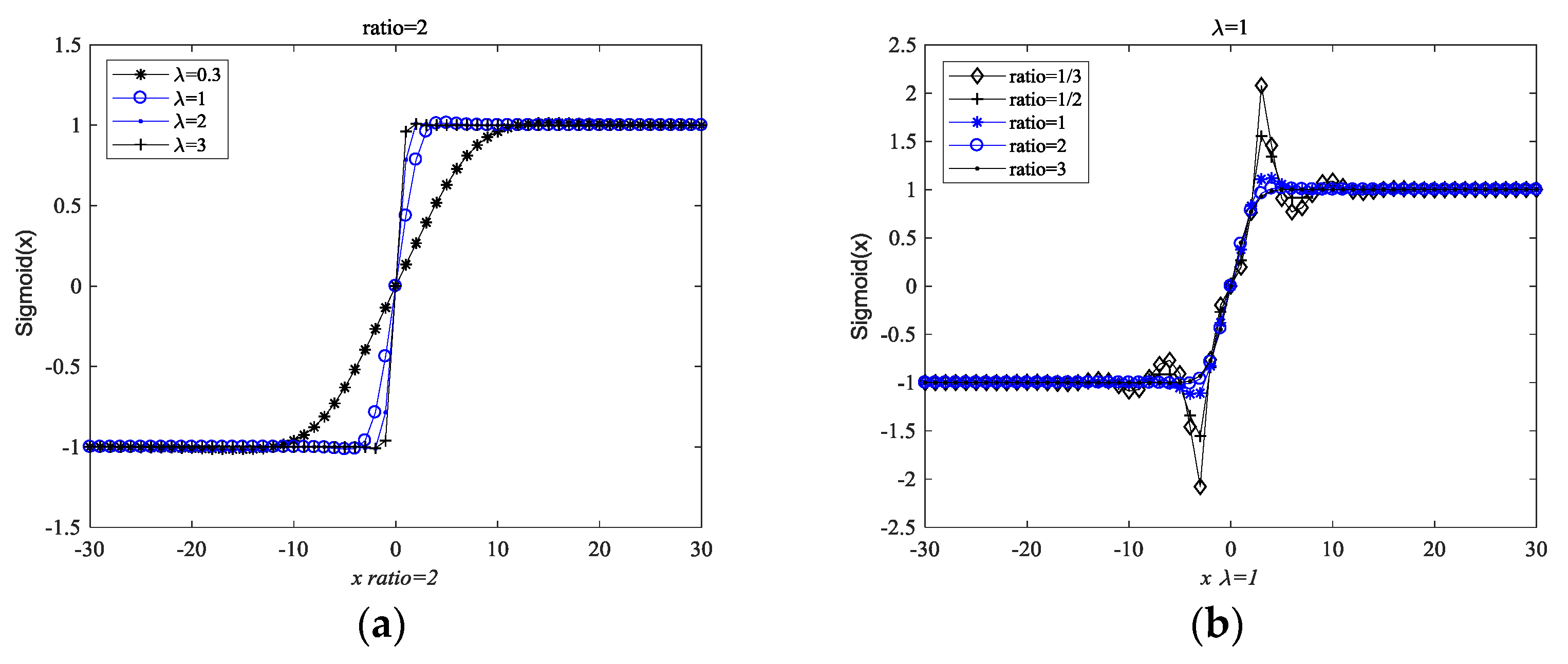
is a complex signal, the above results do not always hold.
Figure 3 demonstrates the Sigmoid function curves of the complex signal with respect to
, and the ratio between the real and imaginary component.
Figure 3a shows that the tuneable Sigmoid function changes with respect to
when the ratio between the real and imaginary components is 2.
Figure 3b shows that the tuneable Sigmoid function changes with respect to
, with the same amplitude, but with a different ratio between the real and imaginary component when the inclined coefficient
is 1. We found that the suppression capability may be increased by increasing the ratio between the real and imaginary components.
We observed that
may not be true when
is a complex signal, as illustrated in
Figure 3. Furthermore, we also found that the amplitude of the complex signal, the inclined coefficient
, and the ratio between the real and imaginary components had some effects in suppressing the impulsive noise capability of the tuneable Sigmoid function.
Figure 4 shows that the suppression ability of the tuneable Sigmoid function for a
noise with
and
. In this simulation, the signal
is the complex signal with impulsive noise. The Sigmoid function employs the tuneable parameter
, which could be used to control the inclination of the curve. The outliers can be suppressed after the transformation. From
Figure 4, we found that the suppression capability may be decreased by increasing the inclined coefficient
, and the tuneable Sigmoid function with
fails to suppress the interference of the
-stable distribution noise. A higher inclined coefficient
had negative impacts on the suppression capability of the impulsive noise. Therefore, the proper selection of
affected accuracy of the estimation.
5.4. Feasibility Analysis of the TS-FPSD
According to Property 4 of the Sigmoid transform, the Sigmoid transform did not change the modulation characteristic of the signal, i.e.,
and
had the same modulation characteristics. The simulation results are illustrated in
Figure 5 below, to verify this property.
From
Figure 5, we found that the LFM signal
and the tuneable Sigmoid transform of the LFM signal
had the same modulation characteristics in the time domain, and the FRFT of the LFM signal
and the FRFT of the tuneable
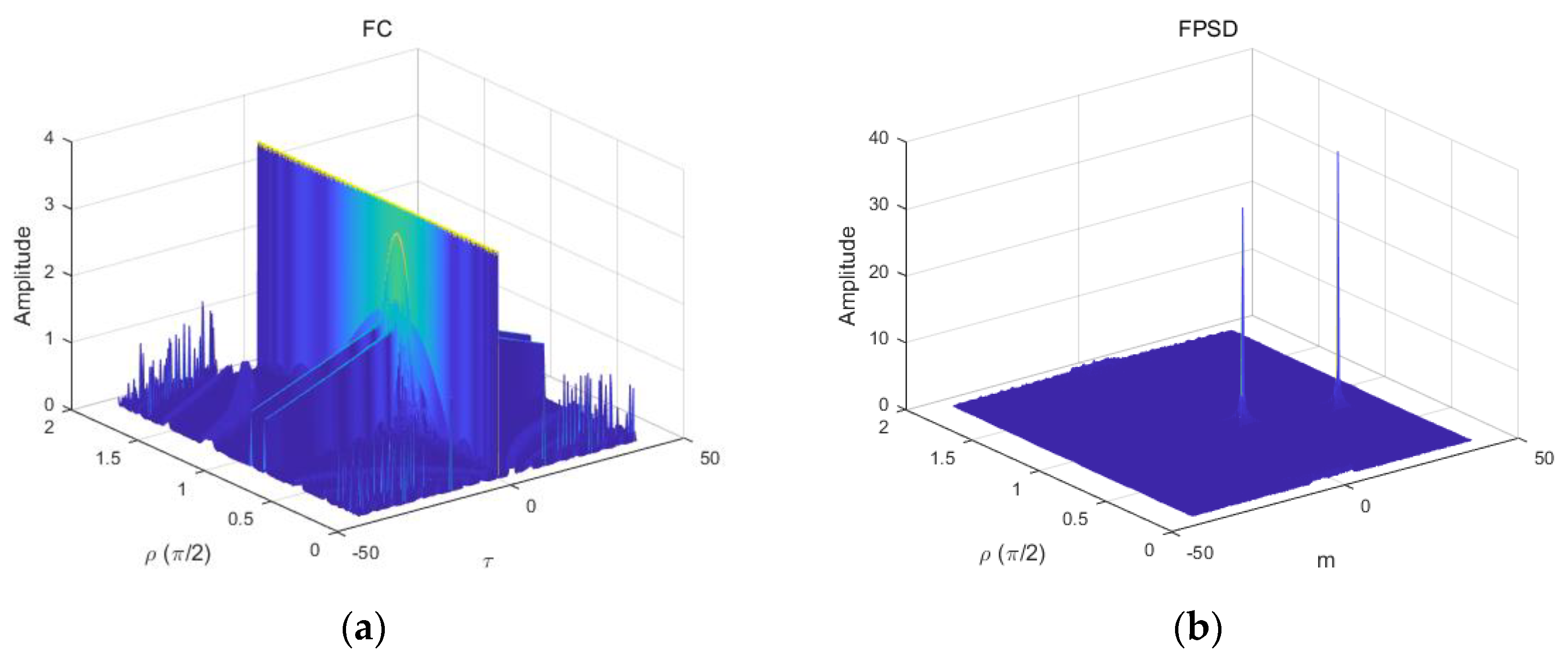
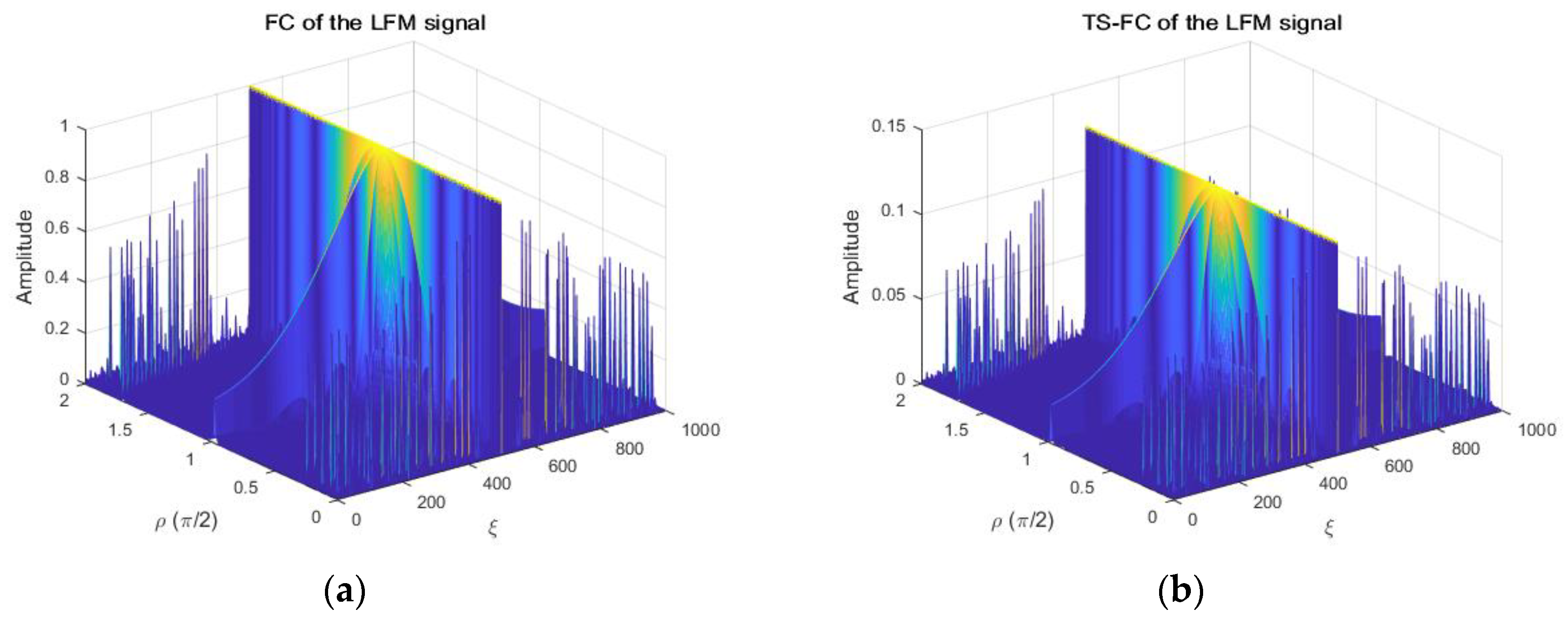
had the same peak locations in the FRFT domain. In conclusion, the tuneable Sigmoid transform did not change the modulation characteristics of the LFM signal. From
Figure 6, we found that the FC of the LFM signal
and the FC of the
had energy concentrations at the same rotation angles in the FRFT domain. The FPSD of the LFM signal and the TS-FPSD of the LFM signal had also the same peak locations in the FRFT domain Moreover, the peak location was the same for the FRFT of the LFM signal and the FRFT of the tuneable
, as illustrated in
Figure 5b,c and
Figure 6b,c. Thus, the Sigmoid transform did not change the modulation characteristics of the signal.
In summary, the parameters of the Doppler stretch and the time delay could be estimated by searching for the peak of the TS-FPSD.
5.5. The Cramer–Rao Bound
In this section, we derived a novel explicit expression for the exact Cramer–Rao Bound (CRB) on the accuracy of estimating the signal model parameters.
The CRB expresses a lower bound for the variance of an unbiased estimate and is, in general, not too difficult to compute. By comparing the performance of an estimator to the CRB, we can often have an indication on how close the estimator is to the optimum.
The echoes signal can be expressed as the following:
where
,
.
The two parameters to be estimated are the time delay and the Doppler stretch , which form the parameter vector , such that ,where denotes the transpose of a vector, , and . Suppose that the number of snapshots is .
First, we obtained closed-form expressions for all particular sub-blocks of the Fisher information matrix (FIM). The element
of the FIM for estimating the vector
can be shown as [
29,
30,
31]:
We assumed that the noise was a sequence of the i.i.d isotropic complex
random variable. The geometric power
is used to represent the power of symmetric
-stable random noise, i.e.,
. Since
and
depend on different elements of
, it is clear that FIM will be block diagonal with respect to the signal (
) and noise parameters. In particular, the first term of Equation (38) will give a nonzero result only for the noise block. Since we are concerned only with the CRB for the signal parameters, we need only consider the second term:
Using Equations (38) and (39), the following explicit expressions for the blocks of the FIM are derived as follows:
where:
The expression for the CRB, shown in Equation (48), is obtained by substituting Equations (40)–(47) into Equation (39):
6. Simulation Results
In this section, we performed four types of simulation experiments to evaluate the relative performances of the FPSD [
12], the FLOS-FPSD [
16], and the TS-FPSD methods under the
-stable distribution noise, respectively.
The parameters of the transmitted LFM signal in the simulation are assumed as follows. The initial frequency
and the modulation rate is set to
. The sampling rate is set to
with a sampling length of
,
T = 1 ms. The number of multipath is
, and the Doppler stretch and time delay are set to
,
,
and
, respectively. The Root Mean Square Error (RMSE) is defined as:
where
and
are the estimation of
and
, and
is the Monte Carlo number. The RMSE of the time delay and Doppler stretch can be expressed as:
and:
The numbers of Monte Carlo runs was set to 200 in Simulations 2 and 3.
Simulation 1: Estimation Accuracy with Respect to
To evaluate the performance of the TD and DS with respect to
in this simulation, the characteristic exponent
was set to
and
. The RMSE was used to evaluate the performance of the TS-FPSD with respect to
, as illustrated is
Figure 7.
From
Figure 7, we observed that the performance estimation of the TD and DS using
provided a better performance than that using other
values, for the case of the alpha-stable noise. Therefore, the inclined coefficient
for the TS-FPSD was set as
in all the later simulations of this paper.
Simulation 2: FPSD, FLOS-FPSD, and TS-FPSD for a Single Estimation
Figure 8 and
Figure 9 show the estimation results of the FPSD, FLOS-FPSD, and TS-FPSD for a single trial of data under the
noise with
and
and
. In order to show the peak location information and the performance of the algorithm more clearly, the 2D rotation angle plane and the 2D frequency plane are shown. The 2D rotation angle plane and 2D frequency plane could better demonstrate the peak location. In
Figure 8 and
Figure 9, the red line denotes the true values of the rotation angle and frequency in the FRFT domain. Futhermore,
Table 1 shows the comparison of three algorithms for impulsive noise suppression.
From
Figure 8a, we found that the FPSD algorithm failed when the
noise occurred. The reason is that the FPSD method did not have the ability to suppress impulsive noise. Since the second-order moment of a
random variable with
does not exist, and the fractional correlation function was based on second-order moments, the performance of the FPSD degraded severely. The FLOS-FPSD algorithm, combining the fractional lower order statistics theory with the fractional power spectrum density function, effectively suppressed the
-stable distribution noise interference, so the FLOS-FPSD could obtain a clear peak under the
noise of
, with
and
. However, the FLOS-FPSD failed to obtain the correct spectrum peak under the
noise with
and
, mainly due to the fact the fractional lower-order moment
value was not appropriate, as illustrated in
Figure 8b,c. In fractional lower order statistics theory, the characteristic exponent of the noise must be estimated to ensure that
or
, otherwise the algorithm performance can degrade seriously, and may even become invalid, while the fractional lower-order moment value is not appropriate.
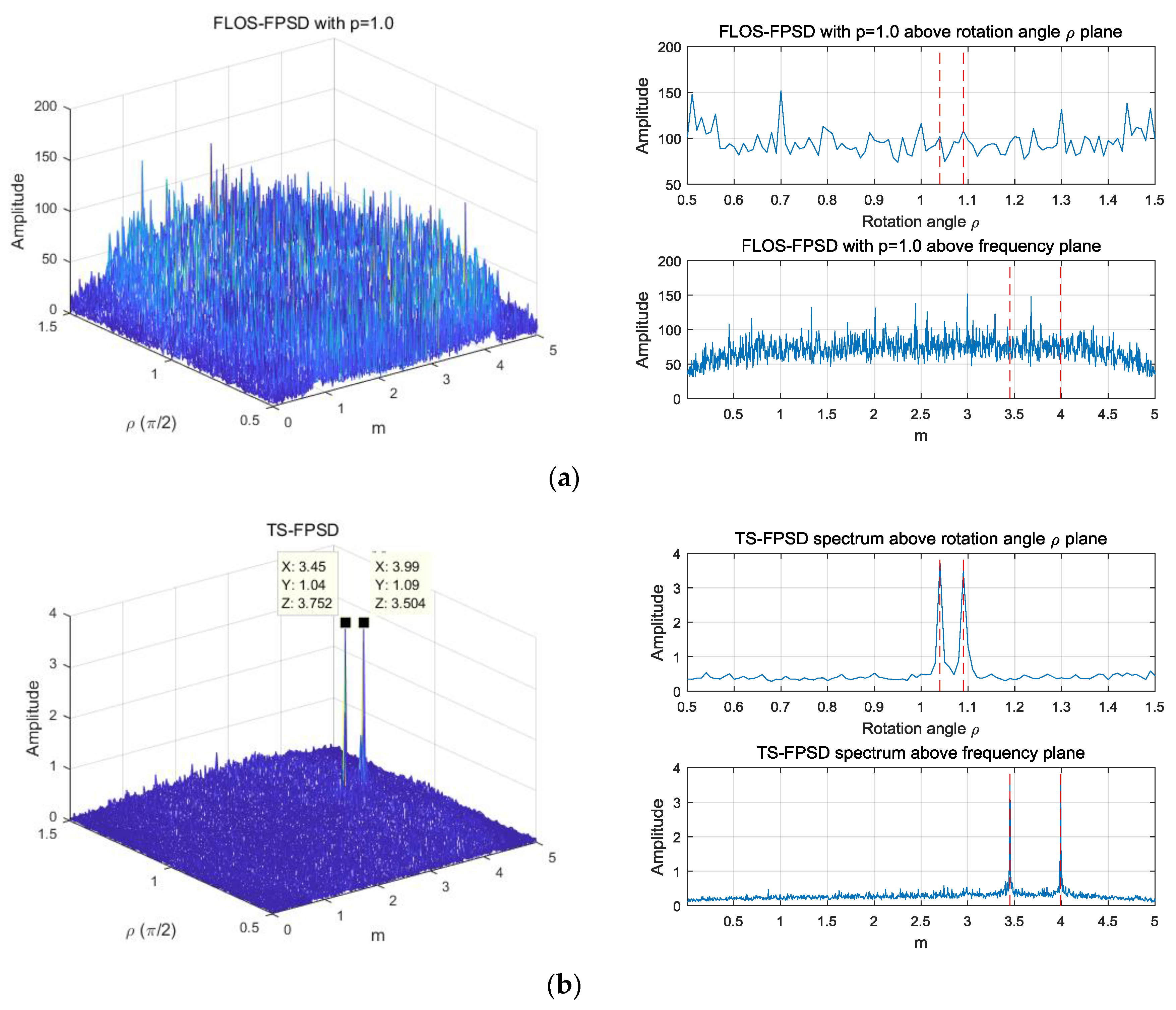
The FLOS-FPSD failed to obtain the correct spectrum peak under the
-stable distribution noise
with
and
; however, the TS-FPSD peak could be easily separated from the impulsive noise, as illustrated in
Figure 9, mainly due to the fact that the Sigmoid transform could suppress the impulsive noise better than the FLOS. Therefore, the performance of the TS-FPSD outweighed those of the FLOS-FPSD. The proposed method based on the TS-FFPSD could effectively suppress impulsive noise interference, yielded an accurate peak estimation, and had a better estimation performance.
Simulation 3: Estimation Accuracy with Respect to GSNR
To evaluate the performance of the time delay (TD) and the Doppler stretch (DS) in this simulation, the characteristic exponent
was set to
and the fractional lower order moment
was set to
and
for the FLOS-FPSD method, respectively. The resulting RMSE performance versus GSNR is illustrated in
Figure 10.
From
Figure 10, we can find that the FPSD method had a poor estimation performance with the
noise interference. On the other hand, combining the fractional lower-order statistics theory with the fractional power spectrum density, the FLOS-FPSD method with
and
could effectively suppress the
noise interference. Accordingly, the FLOS-FPSD method yielded a clear peak under the
noise. However, the performance was affected by the fractional lower-order moment
value. The FLOS-FPSD method, with
and
could not accurately estimate the parameters, because the fractional lower-order moment value was not appropriate. On the contrary, the TS-FPSD method could not suppress the
noise interference, employing the tuneable Sigmoid transform, but the estimation performance of the TS-FPSD also could not be affected by the fractional lower-order moment
value. Therefore, the performance of the TS-FPSD method outweighed those of the FLOS-based method.
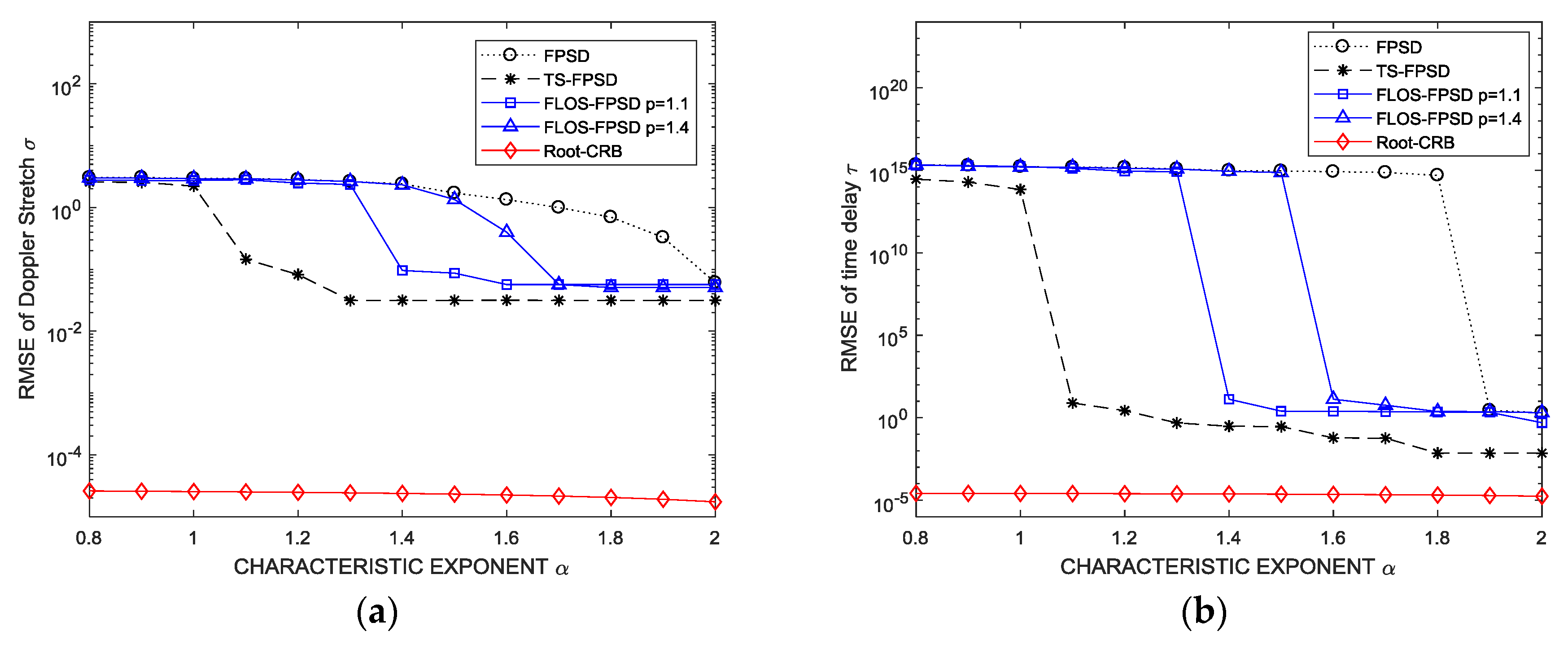
Simulation 4: Estimation Accuracy with Respect to the Characteristic Exponent
In this simulation, the GSNR was set to 5 dB, and the fractional lower-order moment
was set to
and
for the FLOS-FPSD method, respectively.
Figure 11 shows the performance versus the characteristic exponent
. From
Figure 11, we found that the FPSD algorithm had a better estimation performance when the characteristic exponent
was close to 2. The FLOS-FPSD method may suppress the
-stable distribution noise interference by employing the fractional lower-order statistic theory. The performance of the FLOS-FPSD method was shown to be better than that of the FPSD method.
Since the FLOS and the Sigmoid transform methods could both suppress the impulsive noise, the suppression capacity of the FLOS method was not sufficient, and the Sigmoid function suppressed the outliers much harder than did the FLOS. Therefore, the estimation performance of the TS-FPSD algorithm was superior to that of FLOS-FPSD algorithm.


