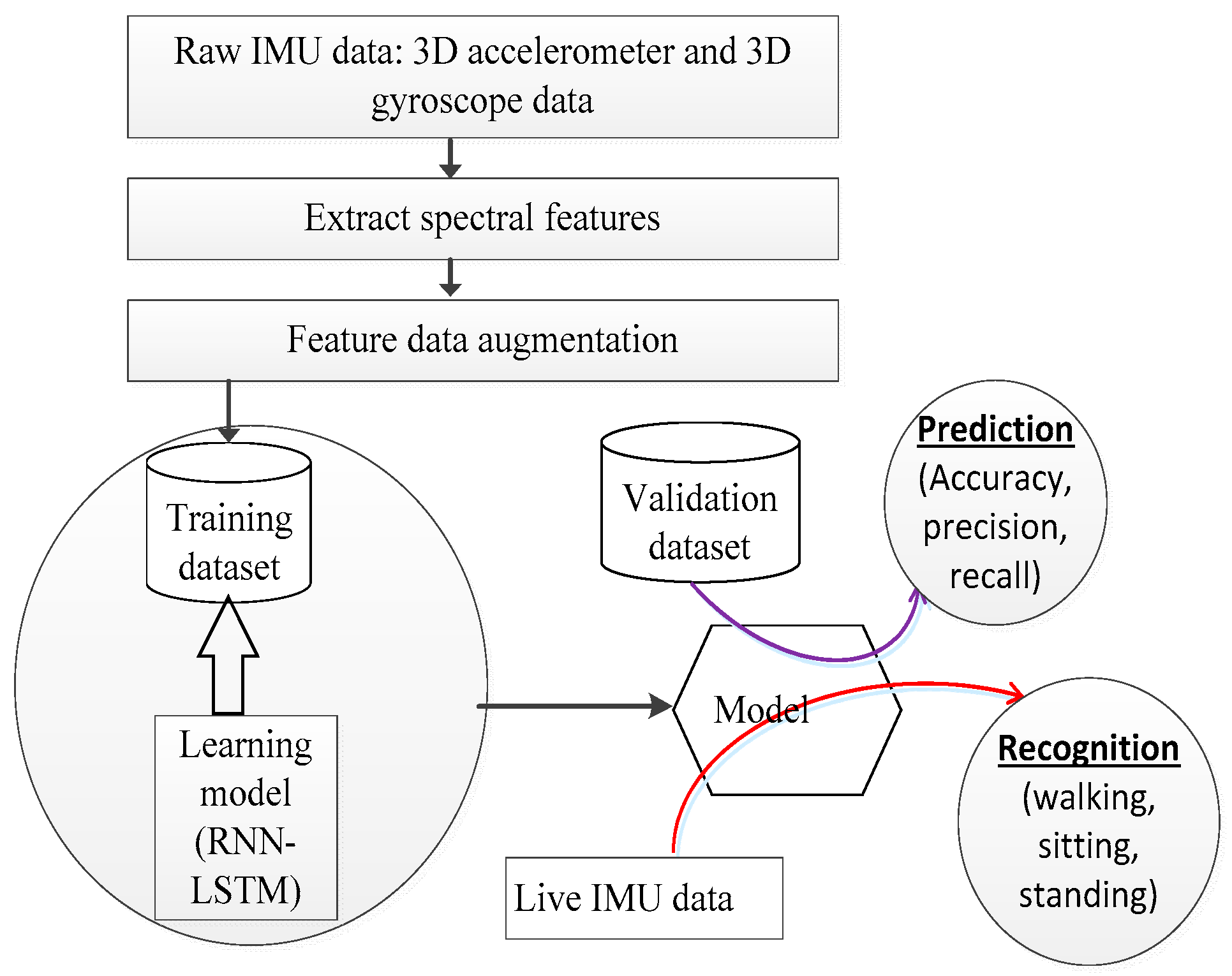
Figure 1.
Human activity recognition system workflow.
Figure 1.
Human activity recognition system workflow.
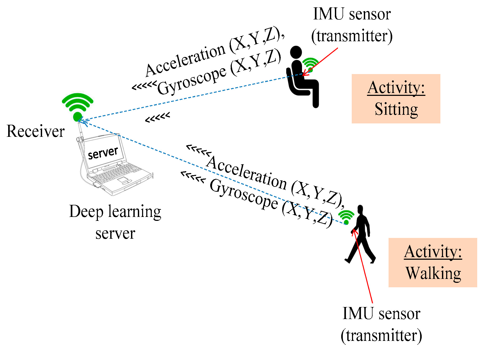
Figure 2.
Data collection architecture.
Figure 2.
Data collection architecture.
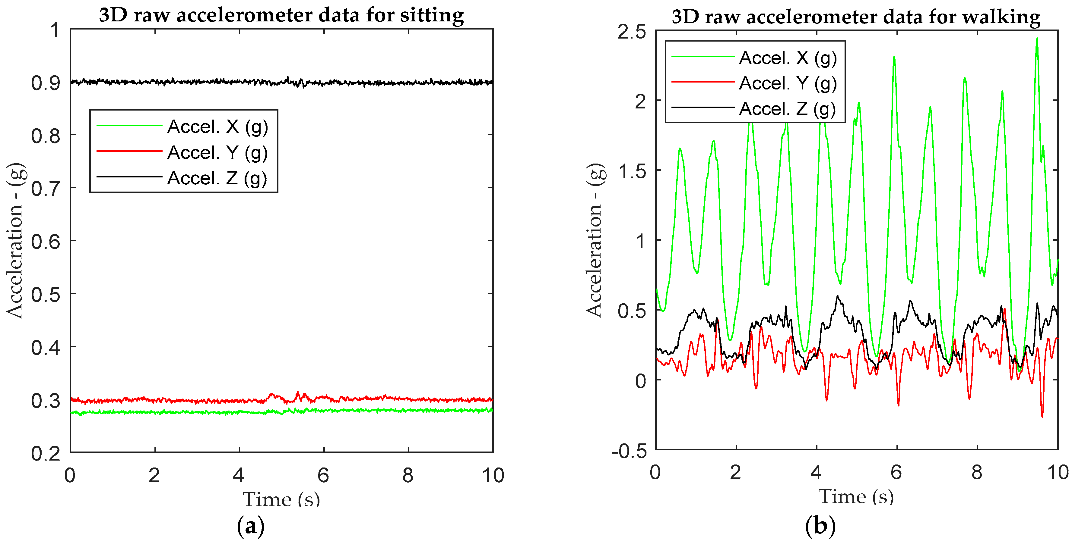
Figure 3.
An example of 3D raw data for (a) sitting and (b) walking based on 1IMU sensor tied on the left-hand wrist.
Figure 3.
An example of 3D raw data for (a) sitting and (b) walking based on 1IMU sensor tied on the left-hand wrist.
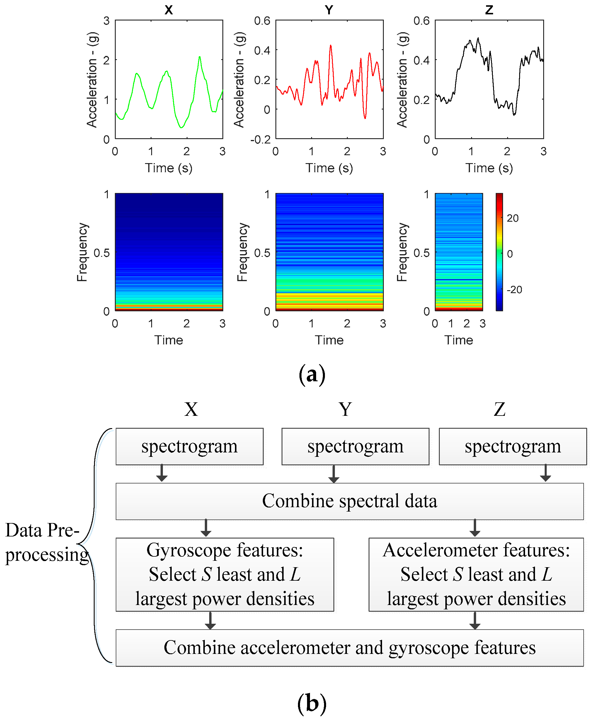
Figure 4.
(a) An example of time domain data and their spectrogram representing walking data; (b) Proposed feature extraction algorithm.
Figure 4.
(a) An example of time domain data and their spectrogram representing walking data; (b) Proposed feature extraction algorithm.
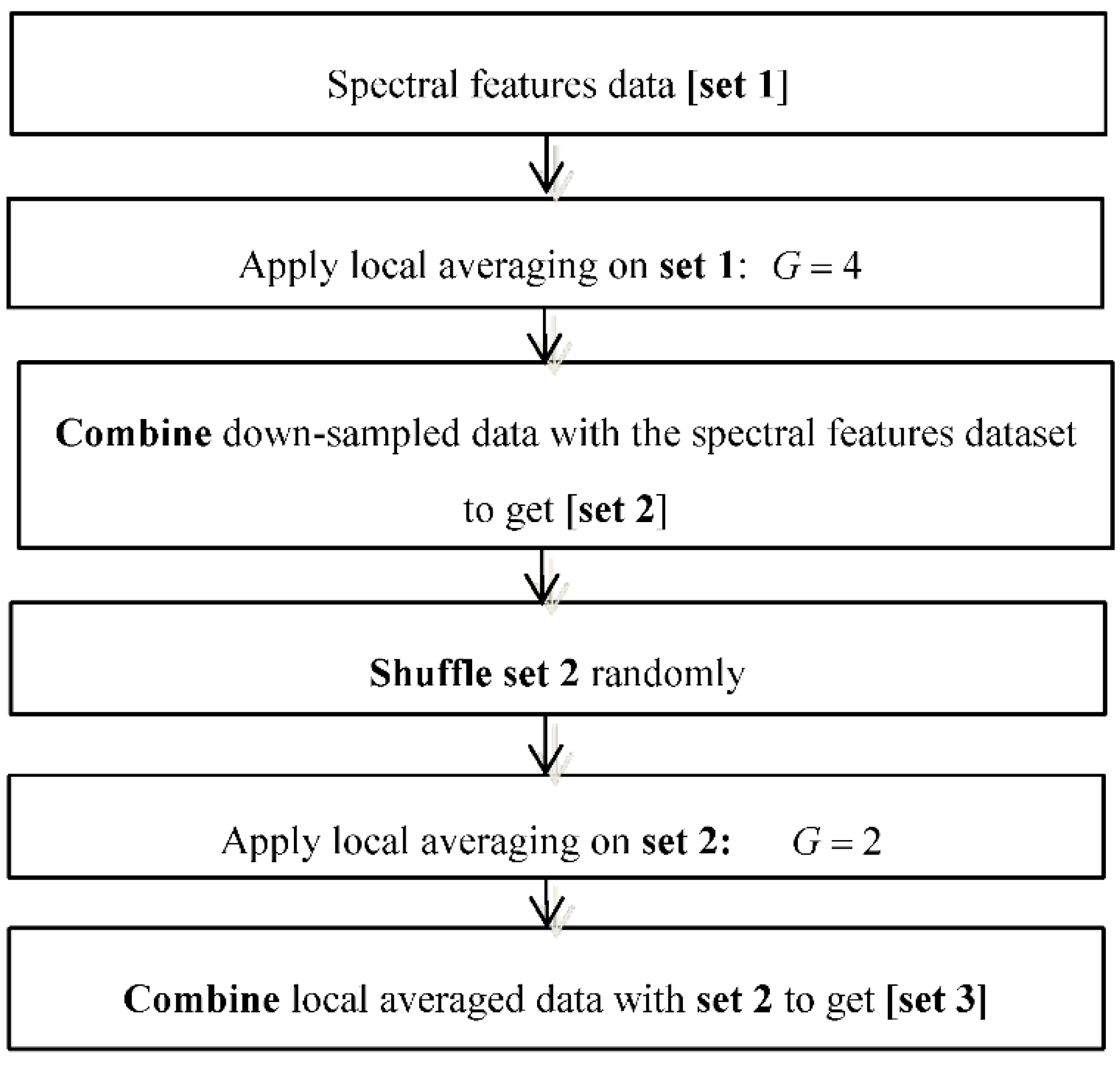
Figure 5.
Data augmentation workflow.
Figure 5.
Data augmentation workflow.
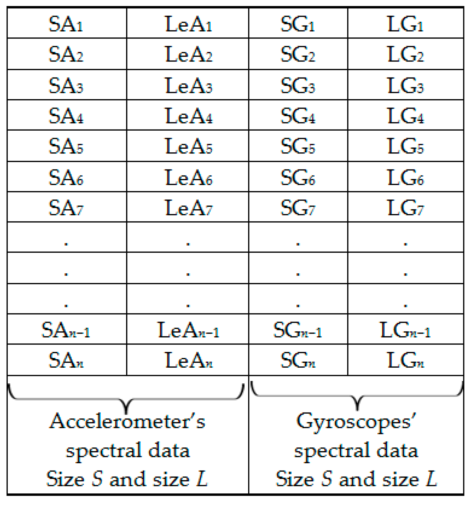
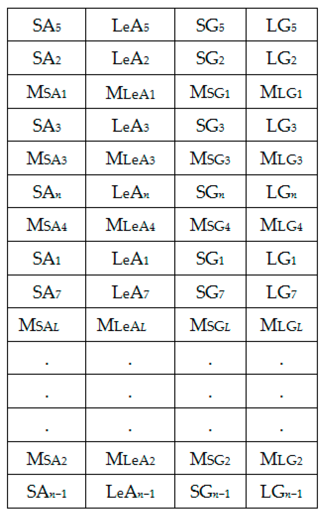
Figure 6.
Set 1: OR dataset.
Figure 6.
Set 1: OR dataset.
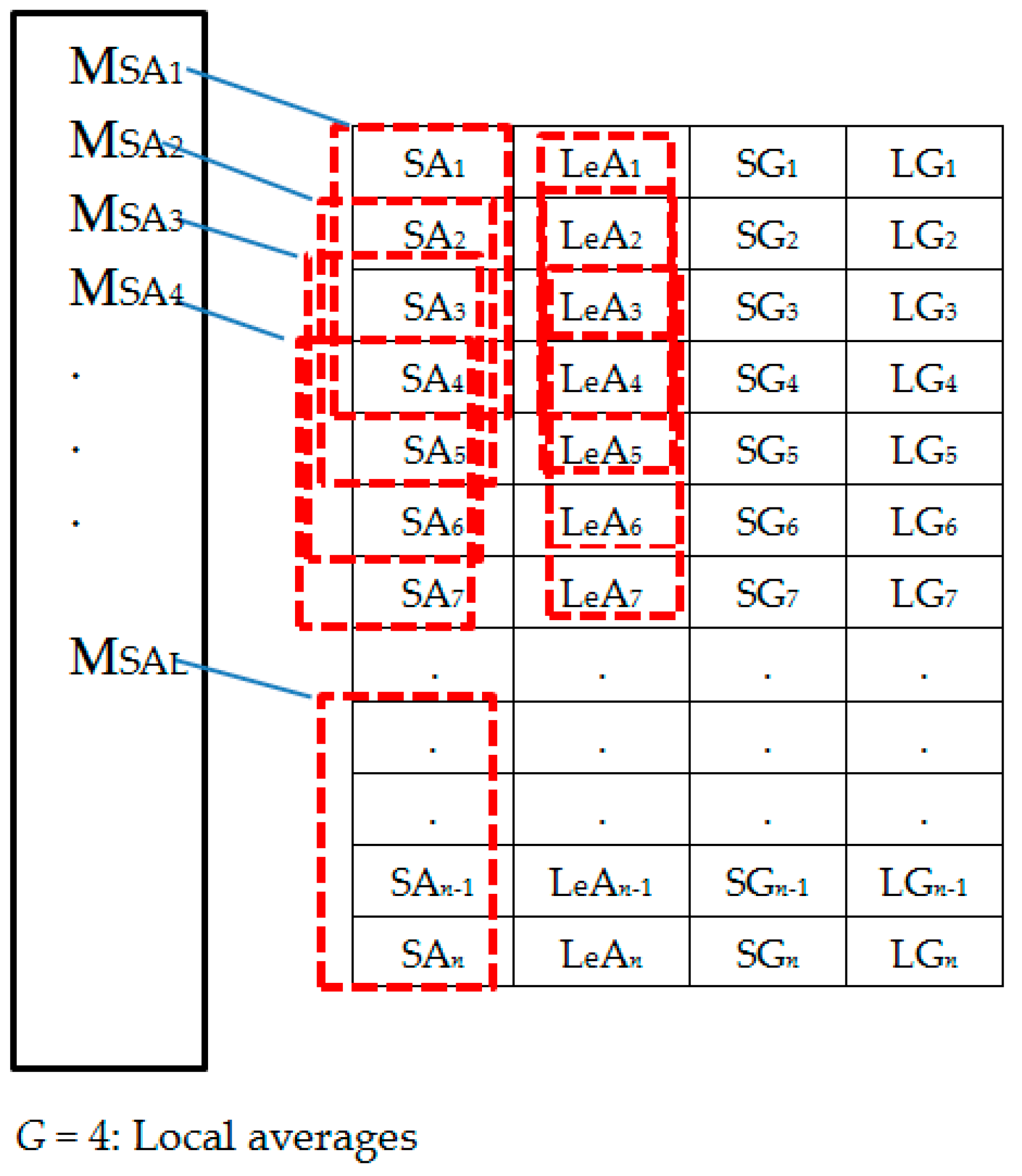
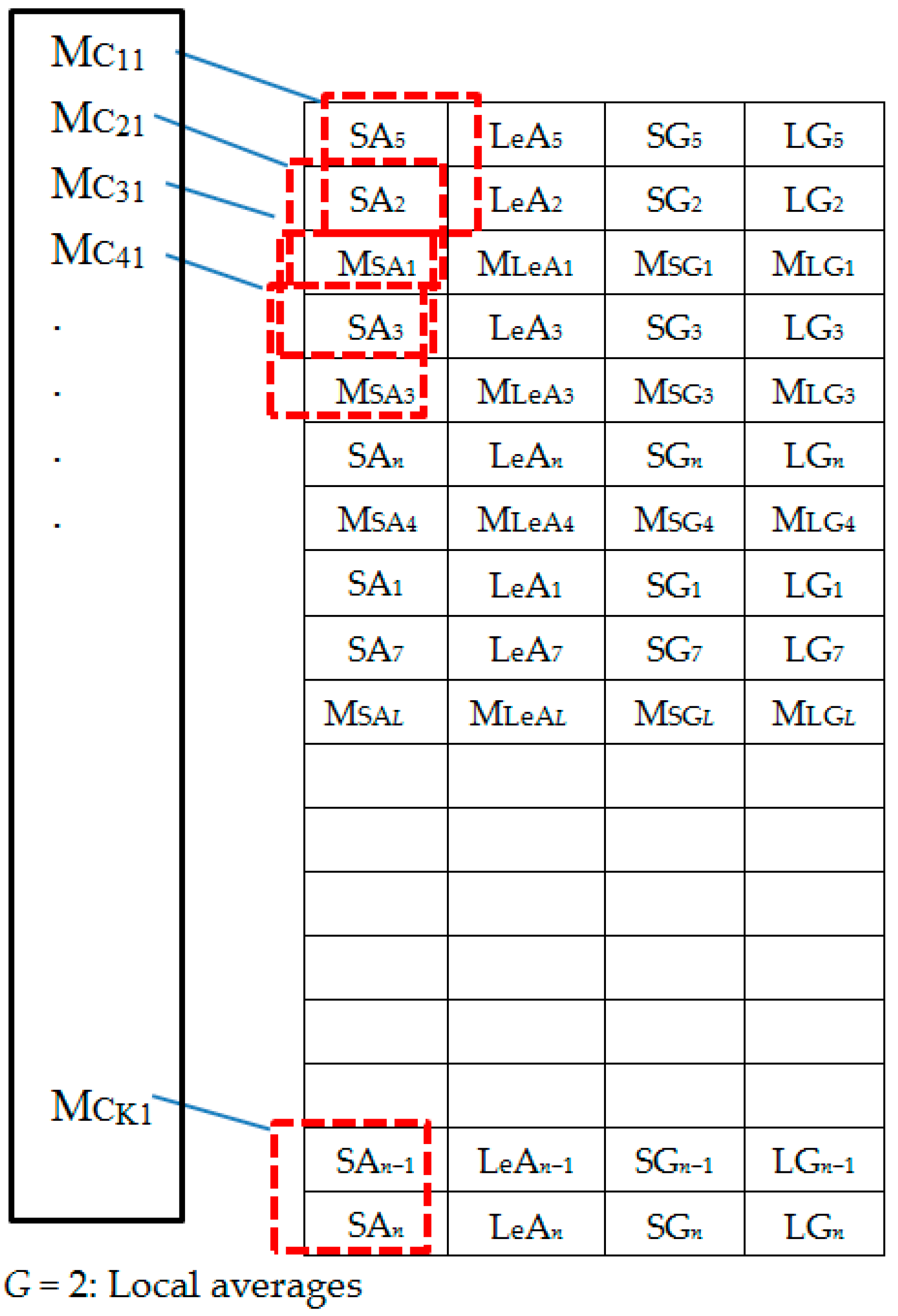
Figure 7.
Set 1: Generating local averages.
Figure 7.
Set 1: Generating local averages.
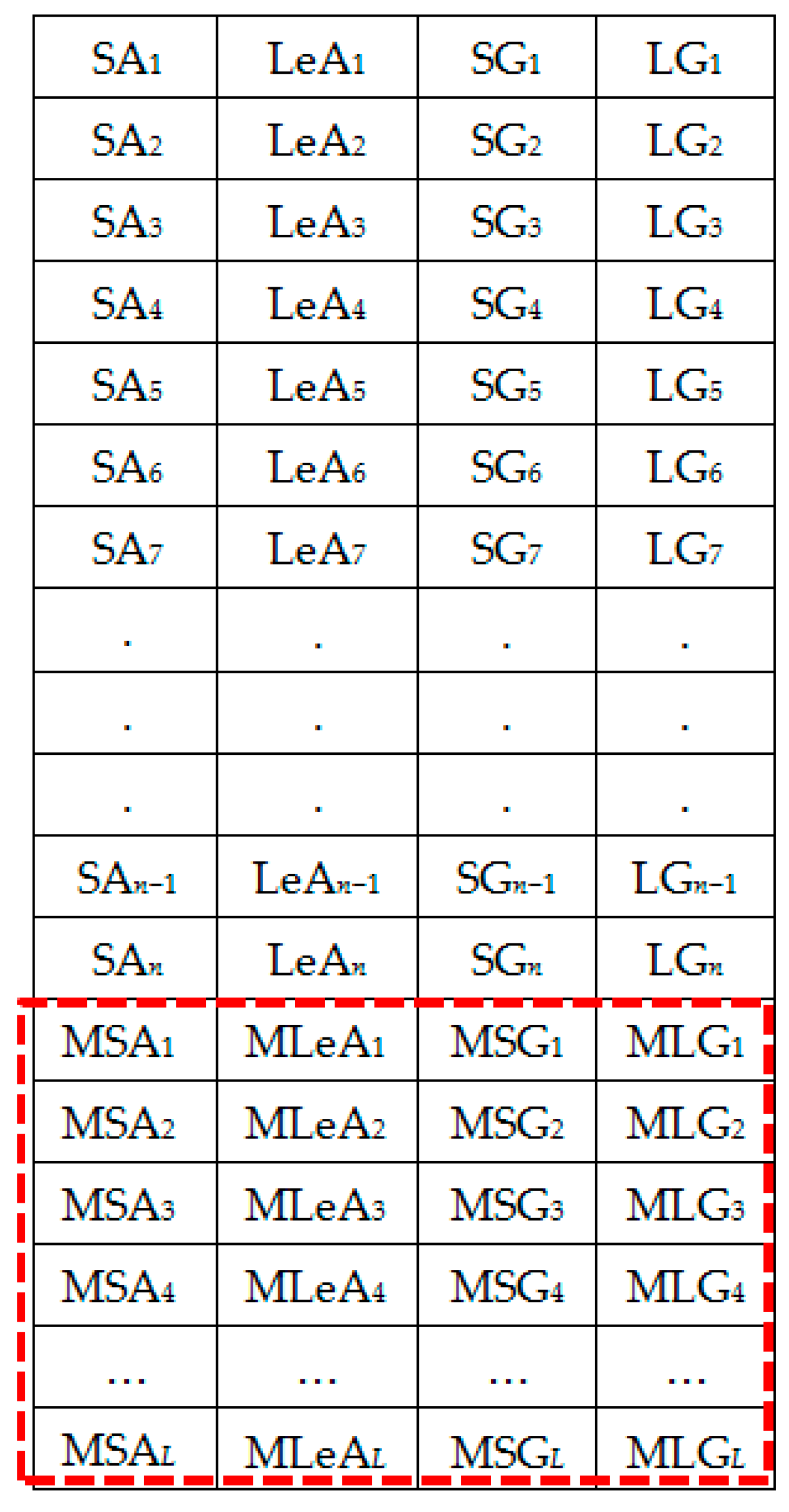
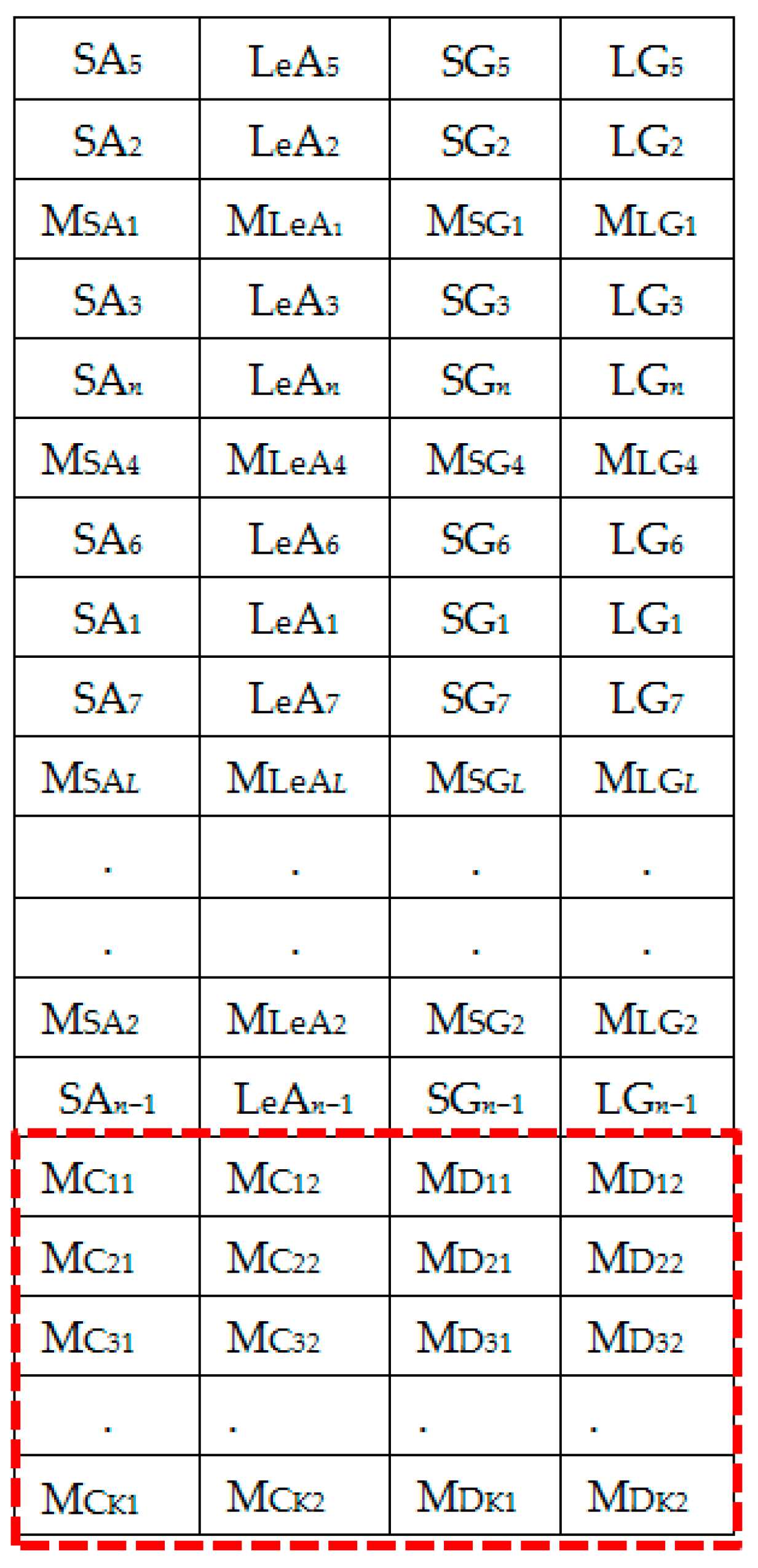
Figure 8.
Set 2: OR + LA1 dataset.
Figure 8.
Set 2: OR + LA1 dataset.
Figure 9.
Randomly shuffled (OR + LA1 + SH) feature set 2.
Figure 9.
Randomly shuffled (OR + LA1 + SH) feature set 2.
Figure 10.
Generating local averages of the shuffled feature set.
Figure 10.
Generating local averages of the shuffled feature set.
Figure 11.
Set 3: OR + LA1 + SH + LA2 feature set with local averages.
Figure 11.
Set 3: OR + LA1 + SH + LA2 feature set with local averages.
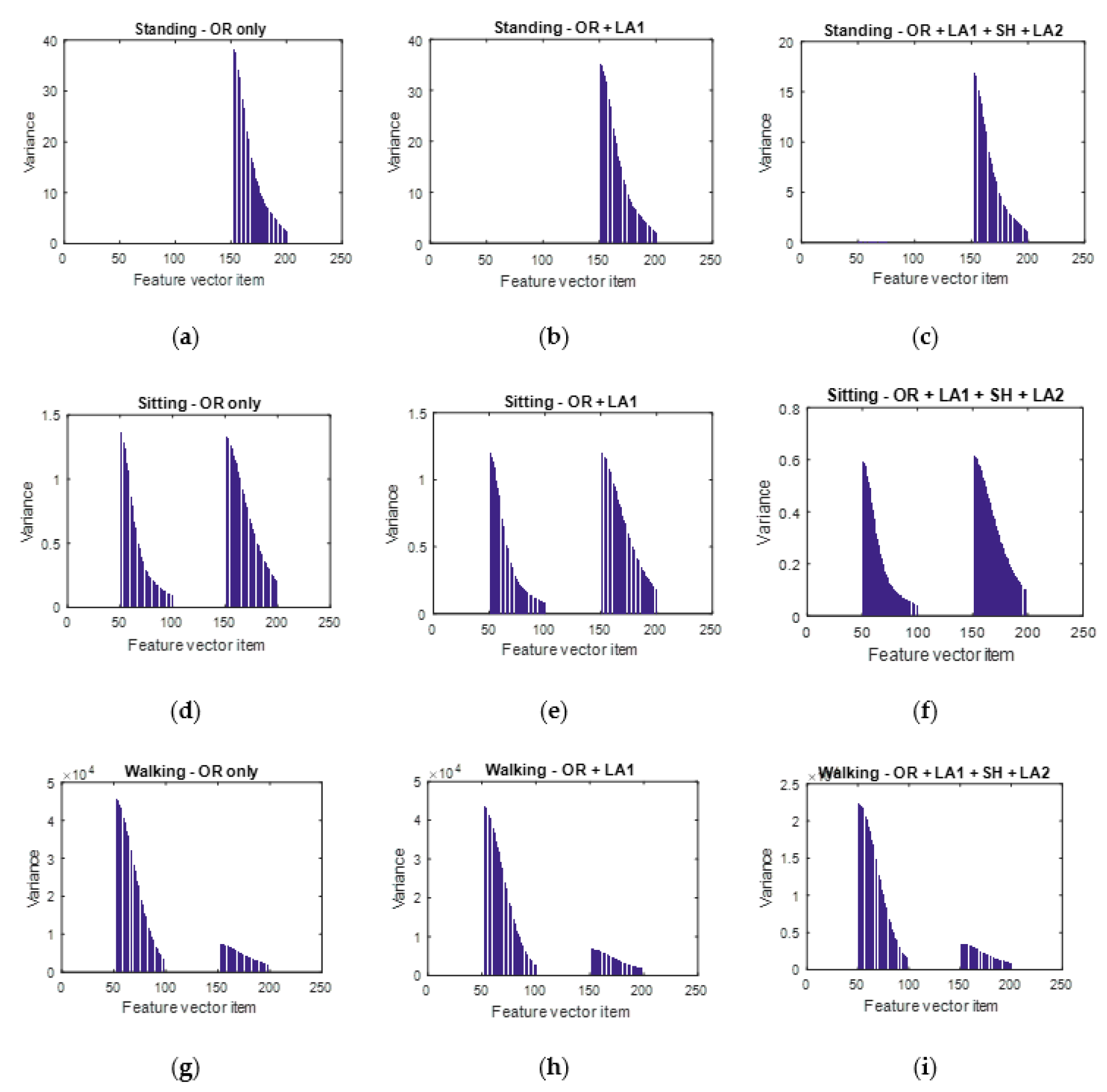
Figure 12.
Visualizing the variance of data to check the influence of each data augmentation block. (a,b,c) represent the variance of the unaugmented dataset, augmented dataset after the first local averaging and that of the augmented dataset after the first local averaging, shuffling and the second local averaging procedure respectively for the standing activity. (d,e,(f) represent the variance of the unaugmented dataset, augmented dataset after the first local averaging and that of the augmented dataset after the first local averaging, shuffling and the second local averaging procedure respectively for the sitting activity. (g,h,i) represent the variance of the unaugmented dataset, augmented dataset after the first local averaging and that of the augmented dataset after the first local averaging, shuffling and the second local averaging procedure respectively for the walking activity.
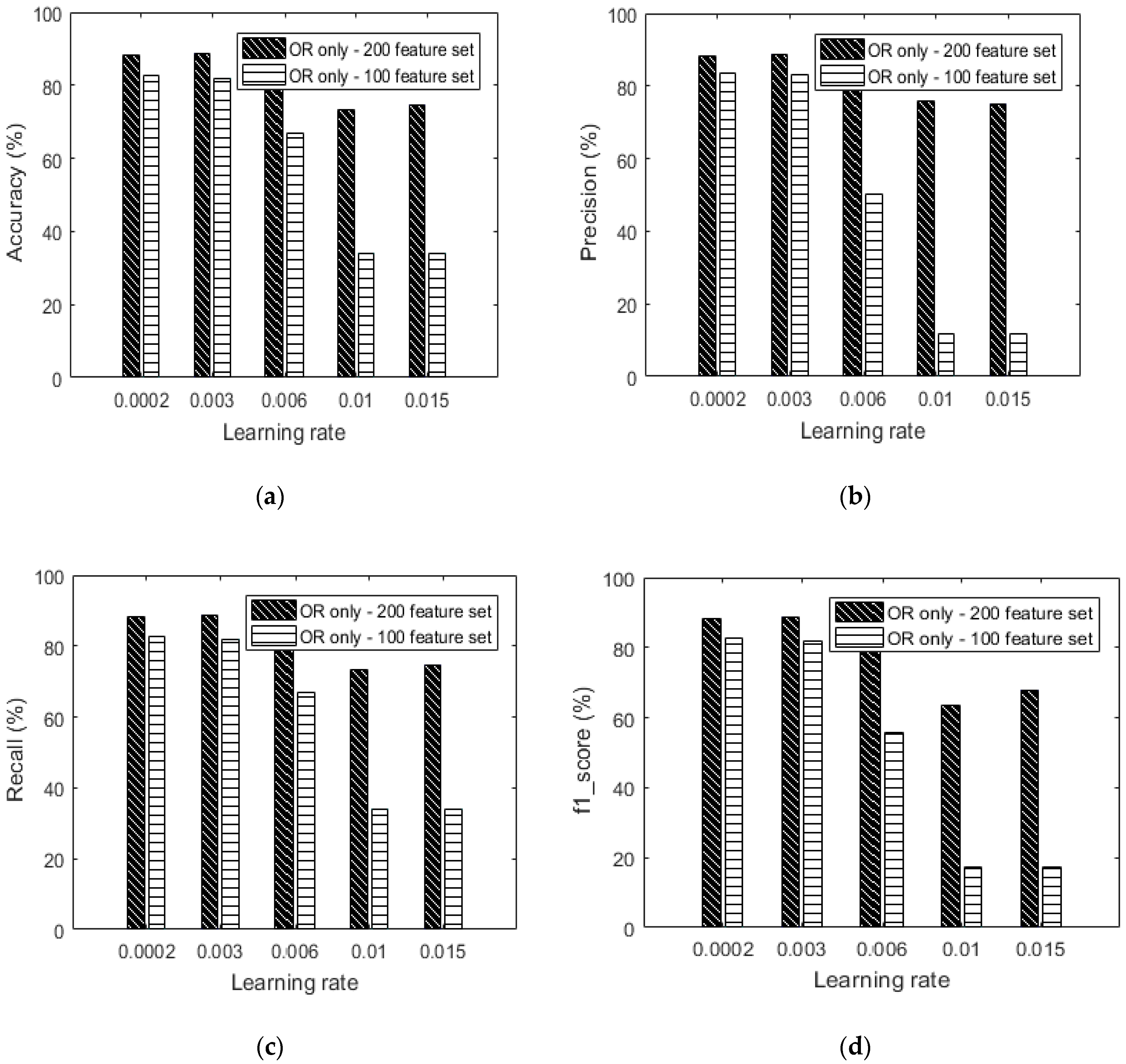
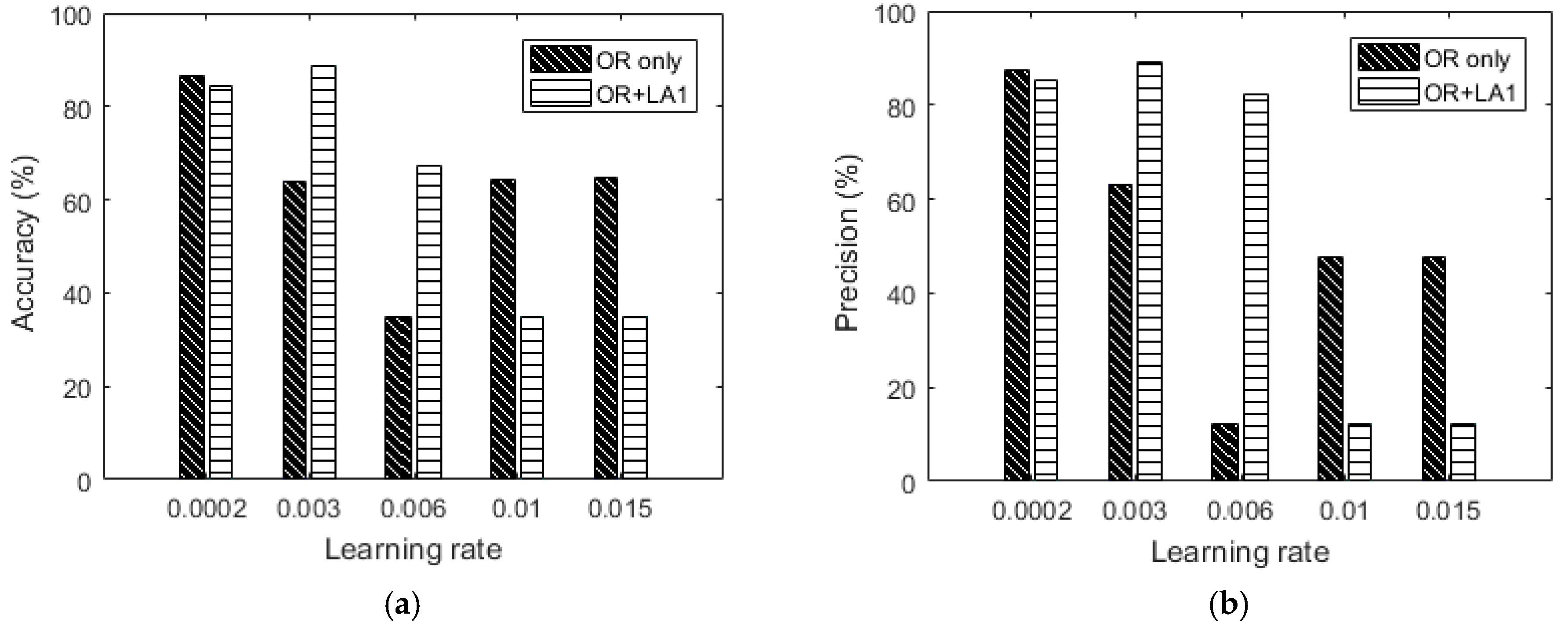
Figure 14.
(a) Accuracy versus learning rate based on only the OR dataset without augmentation, (b) precision versus learning rate based on only the OR dataset without augmentation, (c) recall versus learning rate based on only the OR dataset without augmentation and (d) f1_score versus learning rate based on only the OR dataset without augmentation.
Figure 15.
100-feature vector dataset: (a) Accuracy versus learning rate, (b) precision versus learning rate, (c) recall versus learning rate and (d) f1_score versus learning rate.
Figure 15.
100-feature vector dataset: (a) Accuracy versus learning rate, (b) precision versus learning rate, (c) recall versus learning rate and (d) f1_score versus learning rate.
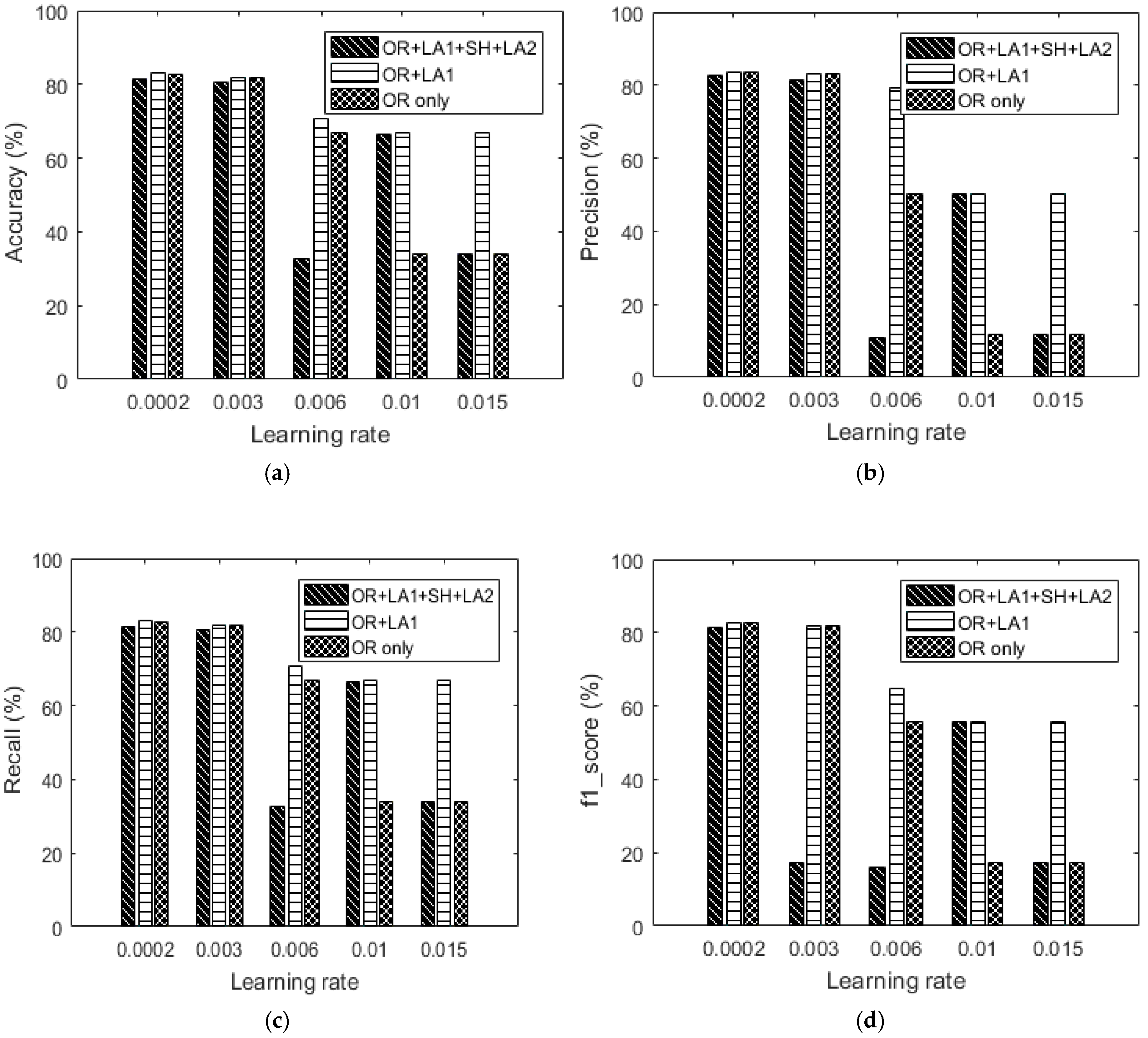
Figure 16.
200-feature vector dataset: (a) Accuracy versus learning rate, (b) precision versus learning rate, (c) recall versus learning rate and (d) f1_score versus learning rate.
Figure 16.
200-feature vector dataset: (a) Accuracy versus learning rate, (b) precision versus learning rate, (c) recall versus learning rate and (d) f1_score versus learning rate.
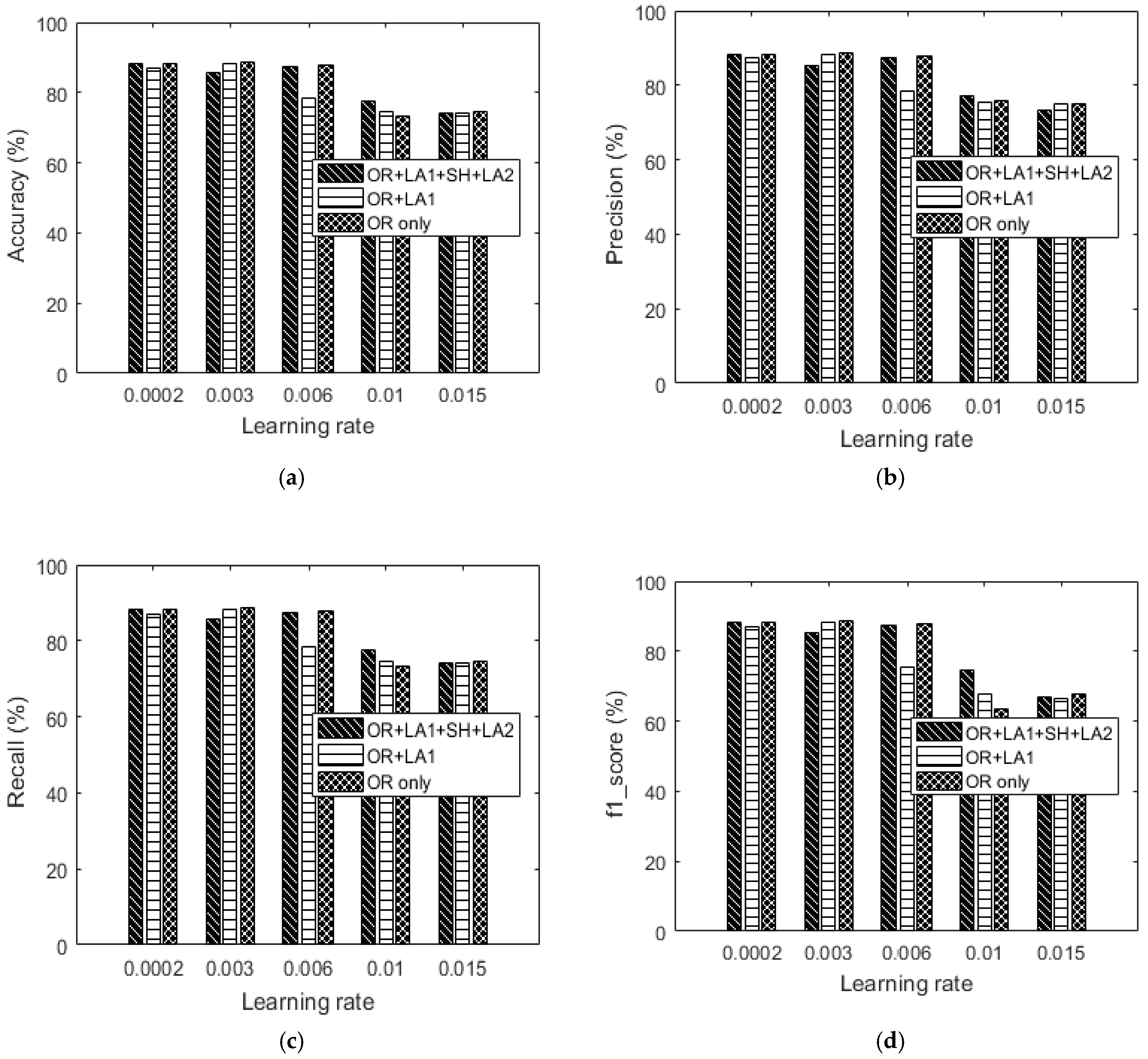
Figure 17.
UCI’s 128-feature vector dataset: (a) Accuracy versus learning rate, (b) precision versus learning rate, (c) recall versus learning rate and (d) f1_score versus learning rate.
Figure 17.
UCI’s 128-feature vector dataset: (a) Accuracy versus learning rate, (b) precision versus learning rate, (c) recall versus learning rate and (d) f1_score versus learning rate.
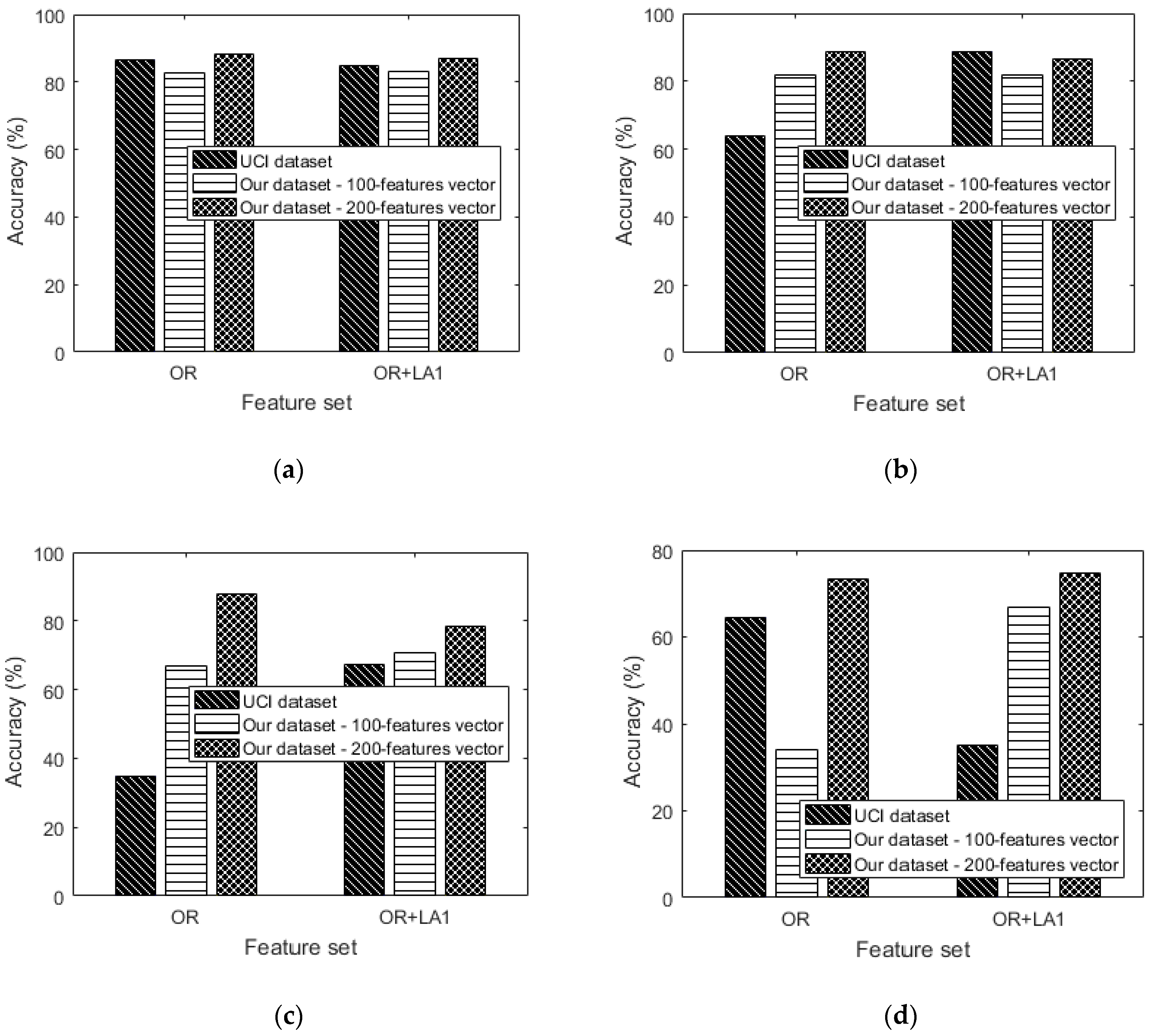
Figure 18.
Comparing the performance of OR and OR + LA1 using the UCI dataset and our dataset at various learning rates of: (a) 0.0002 (b) 0.003 (c) 0.006 and (d) 0.01.
Figure 18.
Comparing the performance of OR and OR + LA1 using the UCI dataset and our dataset at various learning rates of: (a) 0.0002 (b) 0.003 (c) 0.006 and (d) 0.01.
Table 1.
Some of the most widely used features as discussed in [
34].
Table 1.
Some of the most widely used features as discussed in [
34].
| Type | Features | Some Applications |
|---|
| Time-domain | Mean [35], variance, standard deviation [36,37], root mean square [38,39], zero or mean crossing rate [40], derivative, peak counts [41,42] | Human activity recognition [37,38], speech recognition [39], eye movement analysis [42] |
| Frequency-domain | Discrete fast Fourier transforms coefficient, spectral energy [7,43] | Human activity recognition [7] |
| Time frequency domain | Wavelet coefficients [44] | Blink detection [42] |
Table 2.
Performance metrics.
Table 2.
Performance metrics.
| Acronym | Description |
|---|
| Accuracy | The percentage of correctly predicted samples out of the total number of samples. |
| Precision | The fraction of the samples which are actually positive among all the samples which we predicted positive. where, is the number of true positives and is the number of predicted positives. |
| Recall | Measures the proportion of positives that are correctly identified. Where, is the number of true positives and is the actual number of positives. |
| f1_score | The weighted harmonic means of precision and recall. |
Table 3.
Experimental setup.
Table 3.
Experimental setup.
| Description | Value |
|---|
| Number of hidden nodes | 15 |
| Learning rates tested | 0.002, 0.006, 0.003, 0.015, 0.01 |
| Mini batch size | 8000 |
| Loss | 0.001 |
| Regularization | L2 |
| Activation function | RELU (rectified linear unit) |
| Number of training samples (OR + LA1 + SH + LA2) | 9616 |
| Number of training samples (OR + LA1) | 6414 |
| Number of training samples (OR only) | 5132 |
| Number of test samples | 2614 |
| Optimization (back propagation) | Adam optimizer |
Table 4.
Batch size versus accuracy (OR + LA1 + SH + LA2).
Table 4.
Batch size versus accuracy (OR + LA1 + SH + LA2).
| Batch Size | Accuracy |
|---|
| 4500 | 76.95 |
| 4000 | 80.51 |
| 6000 | 82.8 |
| 8000 | 88.14 |
Table 5.
Confusion matrices: (OR only)—100-feature vector datasets.
Table 5.
Confusion matrices: (OR only)—100-feature vector datasets.
| Learning Rate | (a) 0.0002 | (b) 0.006 | (c) 0.003 | (d) 0.015 | (e) 0.01 |
|---|
| True label | ST | 441 | 240 | 0 | 0 | 681 | 0 | 409 | 272 | 0 | 0 | 0 | 681 | 0 | 0 | 681 |
| SI | 113 | 560 | 0 | 0 | 673 | 0 | 98 | 575 | 0 | 0 | 0 | 673 | 0 | 0 | 673 |
| WA | 0 | 1 | 700 | 0 | 2 | 699 | 0 | 1 | 700 | 0 | 0 | 701 | 0 | 0 | 701 |
| | ST | SI | WA | ST | SI | WA | ST | SI | WA | ST | SI | WA | ST | SI | WA |
| Predicted label |
Table 6.
Confusion matrices: (OR only)—200-feature vector dataset.
Table 6.
Confusion matrices: (OR only)—200-feature vector dataset.
| Learning Rate | (a) 0.0002 | (b) 0.006 | (c) 0.003 | (d) 0.015 | (e) 0.01 |
|---|
| True label | ST | 547 | 153 | 0 | 550 | 149 | 1 | 555 | 145 | 0 | 81 | 580 | 39 | 13 | 656 | 31 |
| SI | 154 | 1066 | 0 | 168 | 1052 | 0 | 150 | 1070 | 0 | 33 | 1177 | 10 | 3 | 1207 | 10 |
| WA | 0 | 0 | 694 | 1 | 0 | 693 | 0 | 0 | 694 | 0 | 0 | 694 | 1 | 0 | 693 |
| | ST | SI | WA | ST | SI | WA | ST | SI | WA | ST | SI | WA | ST | SI | WA |
| Predicted label |
Table 7.
Confusion matrices: (OR + LA1)—100-feature vector dataset.
Table 7.
Confusion matrices: (OR + LA1)—100-feature vector dataset.
| Learning Rate | (a) 0.0002 | (b) 0.006 | (c) 0.003 | (d) 0.015 | (e) 0.01 |
|---|
| True label | ST | 437 | 244 | 0 | 97 | 584 | 0 | 416 | 265 | 0 | 0 | 681 | 0 | 0 | 680 | 1 |
| SI | 106 | 567 | 0 | 18 | 655 | 0 | 103 | 570 | 0 | 0 | 673 | 0 | 0 | 673 | 0 |
| WA | 0 | 1 | 700 | 1 | 0 | 700 | 0 | 1 | 700 | 0 | 1 | 700 | 0 | 0 | 701 |
| | ST | SI | WA | ST | SI | WA | ST | SI | WA | ST | SI | WA | ST | SI | WA |
| Predicted label |
Table 8.
Confusion matrices: (OR + LA1 + SH + LA2)—100-feature vector dataset.
Table 8.
Confusion matrices: (OR + LA1 + SH + LA2)—100-feature vector dataset.
| Learning Rate | (a) 0.0002 | (b) 0.006 | (c) 0.003 | (d) 0.015 | (e) 0.01 |
|---|
| True label | ST | 406 | 273 | 2 | 0 | 681 | 0 | 391 | 289 | 1 | 0 | 0 | 681 | 0 | 681 | 0 |
| SI | 91 | 578 | 4 | 0 | 678 | 0 | 102 | 571 | 0 | 0 | 0 | 673 | 0 | 673 | 0 |
| WA | 7 | 2 | 692 | 0 | 701 | 0 | 10 | 0 | 691 | 0 | 0 | 701 | 0 | 8 | 693 |
| | ST | SI | WA | ST | SI | WA | ST | SI | WA | ST | SI | WA | ST | SI | WA |
| Predicted label |
Table 9.
Confusion matrices: (OR + LA1)—200-feature vector dataset.
Table 9.
Confusion matrices: (OR + LA1)—200-feature vector dataset.
| Learning Rate | (a) 0.0002 | (b) 0.006 | (c) 0.003 | (d) 0.015 | (e) 0.01 |
|---|
| True label | ST | 578 | 121 | 1 | 223 | 477 | 0 | 537 | 168 | 0 | 56 | 611 | 33 | 56 | 611 | 33 |
| SI | 219 | 1001 | 0 | 88 | 1132 | 0 | 140 | 1080 | 0 | 21 | 1188 | 11 | 21 | 1188 | 11 |
| WA | 0 | 0 | 694 | 0 | 0 | 694 | 0 | 0 | 694 | 1 | 0 | 693 | 1 | 0 | 693 |
| | ST | SI | WA | ST | SI | WA | ST | SI | WA | ST | SI | WA | ST | SI | WA |
| Predicted label |
Table 10.
Confusion matrices: (OR + LA1 + SH + LA2)—200-feature vector dataset.
Table 10.
Confusion matrices: (OR + LA1 + SH + LA2)—200-feature vector dataset.
| Learning Rate | (a) 0.0002 | (b) 0.006 | (c) 0.003 | (d) 0.015 | (e) 0.01 |
|---|
| True label | ST | 406 | 273 | 2 | 0 | 681 | 0 | 391 | 289 | 1 | 0 | 0 | 681 | 0 | 681 | 0 |
| SI | 91 | 578 | 4 | 0 | 678 | 0 | 102 | 571 | 0 | 0 | 0 | 673 | 0 | 673 | 0 |
| WA | 7 | 2 | 692 | 0 | 701 | 0 | 10 | 0 | 691 | 0 | 0 | 701 | 0 | 8 | 693 |
| | ST | SI | WA | ST | SI | WA | ST | SI | WA | ST | SI | WA | ST | SI | WA |
| Predicted label |
Table 11.
Confusion matrices: (OR + LA1).
Table 11.
Confusion matrices: (OR + LA1).
| Learning Rate | (a) 0.0002 | (b) 0.006 | (c) 0.003 | (d) 0.015 | (e) 0.01 |
|---|
| True label | ST | 455 | 67 | 10 | 525 | 0 | 7 | 471 | 57 | 4 | 532 | 0 | 0 | 532 | 0 | 0 |
| SI | 153 | 337 | 1 | 485 | 1 | 5 | 107 | 383 | 1 | 491 | 0 | 0 | 491 | 0 | 0 |
| WA | 0 | 0 | 496 | 0 | 0 | 496 | 0 | 0 | 496 | 496 | 0 | 0 | 496 | 0 | 0 |
| | ST | SI | WA | ST | SI | WA | ST | SI | WA | ST | SI | WA | ST | SI | WA |
| Predicted label |
Table 12.
Confusion matrices: (OR only).
Table 12.
Confusion matrices: (OR only).
| Learning Rate | (a) 0.0002 | (b) 0.006 | (c) 0.003 | (d) 0.015 | (e) 0.01 |
|---|
| True label | ST | 480 | 48 | 4 | 532 | 0 | 0 | 319 | 210 | 3 | 0 | 528 | 4 | 0 | 530 | 2 |
| SI | 145 | 344 | 2 | 491 | 0 | 0 | 325 | 160 | 6 | 0 | 486 | 5 | 0 | 486 | 5 |
| WA | 3 | 0 | 493 | 496 | 0 | 0 | 0 | 4 | 492 | 0 | 0 | 496 | 0 | 2 | 494 |
| | ST | SI | WA | ST | SI | WA | ST | SI | WA | ST | SI | WA | ST | SI | WA |
| Predicted label |


