Article

Non-Contact Measurement of the Surface Displacement of a Slope Based on a Smart Binocular Vision System

1
School of Civil Engineering and Architecture, Southwest Petroleum University, Chengdu 610500, China
2
School of Transportation and Logistics, Southwest Jiaotong University, Chengdu 610031, China
*
Author to whom correspondence should be addressed.
Sensors 2018, 18(9), 2890; https://doi.org/10.3390/s18092890
Submission received: 14 July 2018 / Revised: 18 August 2018 / Accepted: 25 August 2018 / Published: 31 August 2018
(This article belongs to the Section Physical Sensors)

Abstract

:
The paper presents an intelligent real-time slope surface deformation monitoring system based on binocular stereo-vision. To adapt the system to field slope monitoring, a design scheme of concentric marking point is proposed. Techniques including Zernike moment edge extraction, the least squares method, and k-means clustering are used to design a sub-pixel precision localization method for marker images. This study is mostly focused on the tracking accuracy of objects in multi-frame images obtained from a binocular camera. For this purpose, the Upsampled Cross Correlation (UCC) sub-pixel template matching technique is employed to improve the spatial-temporal contextual (STC) target-tracking algorithm. As a result, the tracking accuracy is improved to the sub-pixel level while keeping the STC tracking algorithm at high speed. The performance of the proposed vision monitoring system has been well verified through laboratory tests.

1. Introduction

Landslide disasters cause serious damage to human life and the economy. Surface deformation is an important basis for assessing the safety status of a slope. At present, slope surface deformation monitoring methods are of five main classes: geodetic methods, global positioning system (GPS) technology, three-dimensional (3D) laser scanning, interferometric synthetic-aperture radar (INSAR) technology, and digital photogrammetry. Geodetic measurement [1] is a traditional monitoring method; however, owing to a low observation frequency and low intelligence, it is difficult to obtain monitoring data that has spatial-temporal continuity. GPS [2] has a high degree of intelligence and can achieve full-time monitoring; however, its target setting is limited, that is, no obstacles are allowed within a range of 15° around the elevation angle of the station in most cases [3]. Both 3D laser scanning [4] and INSAR technology [5] are free at the selection of the marker points, but are costly and difficult to apply to slopes covered with vegetation.
In view of the above problems, owing to their non-contact and cost-effective features, vision-based digital photogrammetry systems have been studied extensively in recent years. The method converts the image coordinates into spatial coordinates by tracking the target image, and obtains the structural deformation information [6]. In practice, the most prominent limitation of visual sensor systems is the measurement accuracy. The main factors affecting this accuracy are (1) marker points and (2) target tracking and positioning. On the one hand, some scholars have used natural marking points when applying machine vision technology to structural deformation monitoring. For instance, Yoon et al. [7] use the Harris corner detection algorithm to extract the feature points of the specified area of a structure. Khuc et al. [8] use a Hessian matrix [9,10] to extract the key points on a steel beam. At the same time, others directly use obvious features such as a light-emitting diode lamps [11] and structural bumps [12,13,14] as the monitoring markers. On the other hand, target markers with specially designed features, such as a circle [15,16,17], a checkerboard [18,19,20], or a random pattern [21], have also been widely used. The position of a feature can be detected and then transformed into the coordinate information. Considering the insufficient feature points of a large slope, it is necessary to artificially set the landmarks to achieve a measurement. The positioning accuracy of the landmarks greatly determines the accuracy of the monitoring results. Common image positioning methods include the least squares fitting method [22], grey weighted centroid method [23], SUSAN algorithm [24], and Hough transform method [25]. Therefore, the authors propose a concentric marker and positioning method that adapts to the visual monitoring system applied. Even if the slope is covered by vegetation, high-precision positioning of the measuring point can be achieved.
For continuous intelligent monitoring, consumer-level cameras can be used to track and locate the landmarks in each frame. The current tracking algorithms mainly include KLT [7,26], CN [27], KCF [28], ODFS [29], and spatial-temporal contextual (STC) [30,31]. However, existing target-tracking algorithms have mostly been studied with regard to their intelligent stability, whereas a few have been studied for their positioning accuracy. To meet the accuracy requirements of deformation monitoring, scholars usually use template matching technology to obtain high-precision monitoring results. A variety of methods are applied to template matching for vision sensors including digital image correlation, pattern matching, optical flow, sub-pixel Hough transforms, random sample consensus, edge detection, sum of squared differences, scale-invariant feature transform, and the orientation code matching(OCM) [14,16,20,32,33,34,35]. Based on the OCM template matching algorithm, Feng et al. [14] demonstrated the high accuracy of the vision sensor for dense full-field displacement measurements through experimental results. Javh et al. [34] showed a sub-pixel displacement resolution of less than thousandths of a pixel by a simplified gradient-based optical flow method under laboratory conditions. However, these methods are limited in obtaining the three-dimensional deformation of a structure. It is generally known that slope surface monitoring requires three-dimensional information. Based on binocular stereoscopic vision measurement technology, to overcome the original frame-by-frame selection method for targets, we combine the temporal-spatial contextual visual tracking algorithm (STC) [31] with sub-pixel image registration technology [36], and improve the tracking accuracy to the sub-pixel level while maintaining the high speed STC algorithm to achieve real-time monitoring.
In this paper, to realise the intelligent real-time monitoring of a slope surface deformation, binocular stereo-vision measurement technology is introduced into the monitoring of the slope surface deformation, and the designs of concentric landmark points and high-precision image positioning methods are described. At the same time, the existing tracking technology is improved to achieve high-precision target tracking and spatial positioning. Finally, laboratory tests conducted to verify the validity and accuracy of the proposed method are detailed.

2. Proposed Smart Binocular Vision System

2.1. Overview

A binocular vision based displacement measurement system is typically composed of hardware and software (see Figure 1). The hardware components consist of a commercial binocular camera, a computer for storing and processing data, and a custom target. The binocular camera has a zoom lens from 4 mm to 12 mm, with a maximum resolution of 2560 × 960 pixels, and an adjustable acquisition frame rate up to 60 fps. The stereo baseline can be adjusted from 4.5 cm to 18 cm, and the field of view of the camera is from 29° to 78°. The vision system was worked on a laptop (Lenovo Xiaoxinchao500, Beijing, China) with an Intel i7-7500U processor with 4 GB of RAM and a mechanical hard disk drive. The movements of a target can be recorded and tracked by the camera and synchronously transferred to the computer, where the displacement is calculated using object centre location algorithms and coordinate transformations.

2.2. Target Design

Visual measurement technology is based on marker imaging. It must be clear that the precise positioning of an object requires searching for obvious feature points. Natural targets are often used in low-precision or near-distance measurements, whereas artificial targets are often used in high-precision or long-distance measurements, particularly for large-scale outdoor engineering structures such as slopes. In this chapter, the design and positioning methods of existing mark points are proposed to achieve the high-precision positioning of the measuring points.

2.2.1. Design Scheme

A round mark point is one of the most common forms of feature points in monitoring. However, a circle shows an elliptical shape after a perspective projection in computer vision imaging. In general, region- and edge-based technologies are used in elliptical centre positioning. The former is inefficient in terms of its operation, and has difficulty ensuring the noise removal effect, and thus it cannot adapt to the complex environment of a slope-engineering site. Instead, the latter can effectively avoid these problems [37]. Therefore, this study uses edge-based elliptical centre positioning technology.
Ellipse fitting technology has been widely used owing to its good fault tolerance, adaptive noise environment, and high efficiency in achieving centre positioning. The basis of the ellipse fitting technique is to obtain the edge information of an image. This study uses sub-pixel edge detection technology to achieve high-precision edge extraction, providing the best edge information for the centre positioning.
After obtaining the centre coordination of each circular mark, the clustering algorithm is used to gain the representative value of the centre of the circle, avoiding the influence of singular values and random errors on the centre orientation.

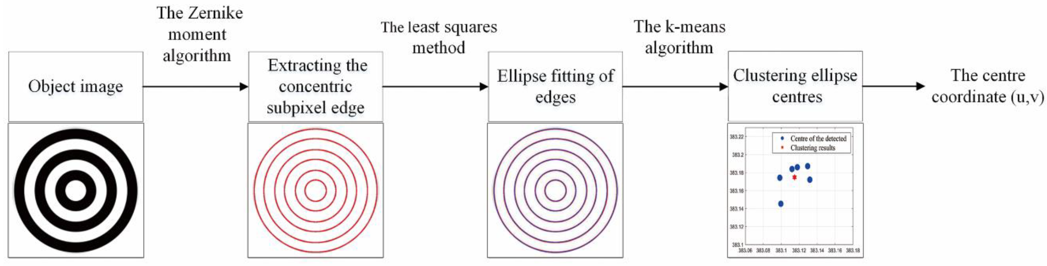
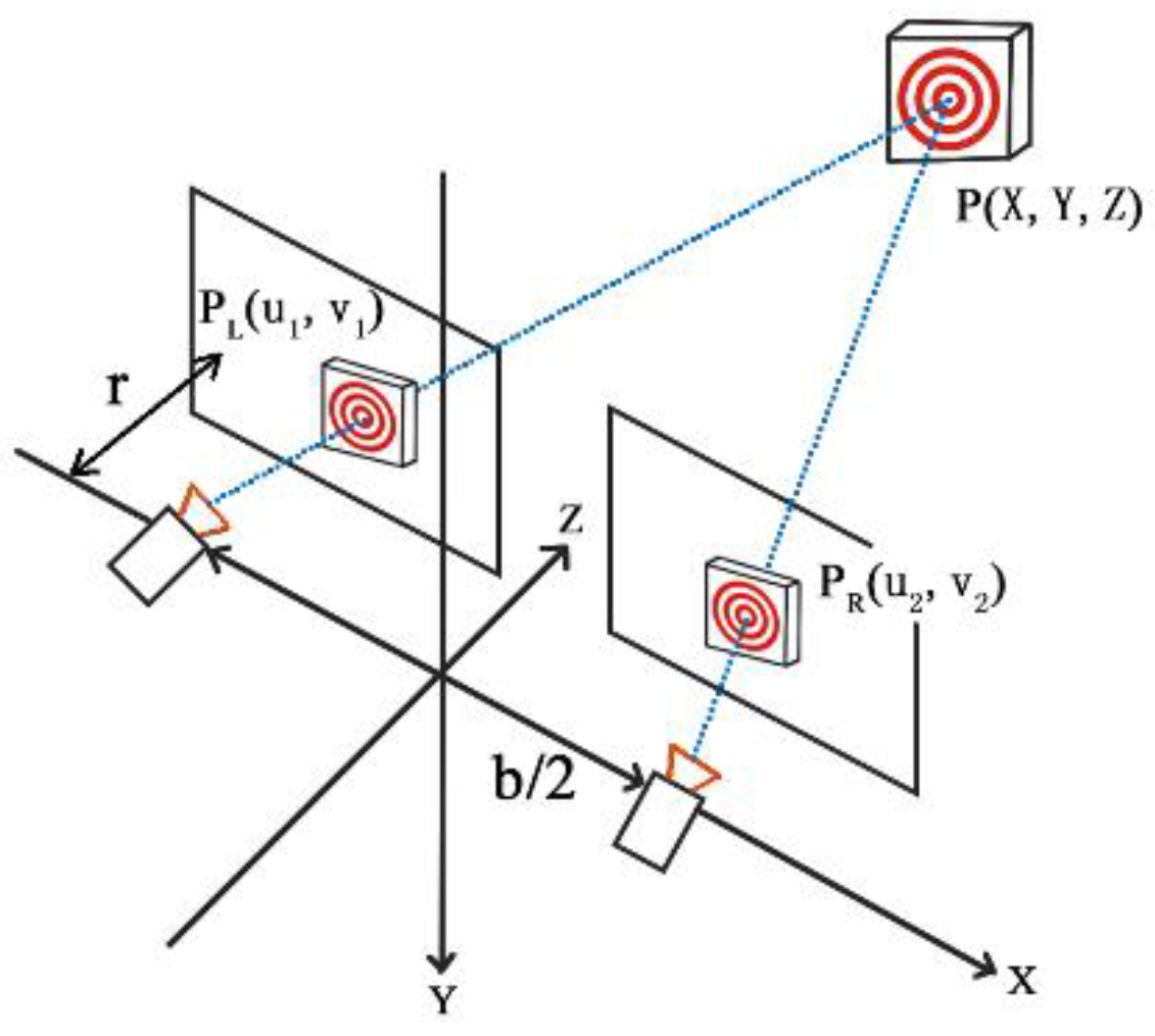
2.2.2. Object Positioning Method

Remote monitoring requires higher accuracy. This study uses the modified template of Gao et al. [38] to extract concentric sub-pixel edges, the basic principle of which is as follows: calculate the edge parameters according to the rotational invariance of the Zernike moment, and use the edge parameters to determine whether it is an edge to accurately extract the edge position. An ellipse is then fitted using the least squares method [39] to locate the centre coordinates of each concentric circle:
x c = b e 2 c d 4 a c b 2 y c = b d 2 a e 4 a c b 2
a, b, c, d, e are the coefficients of the general equation of the ellipse a x 2 + b x y + c y 2 + d x + e y + f = 0 , and f is a constant. Finally, the value of the centre is extracted based on the k-means clustering algorithm [40]. The basic principle lies in the optimisation of the following formula:
J = n = 1 N k = 1 K r n k x n μ k 2
In this equation, N represents the number of data samples; K is the number of clusters; r n k represents 1 when data point n is assigned to class k , and is 0 otherwise; x n indicates the sample data object; and μ k is the cluster centre.
The method in this study achieves the function of target centre location through programming (see Figure 2).

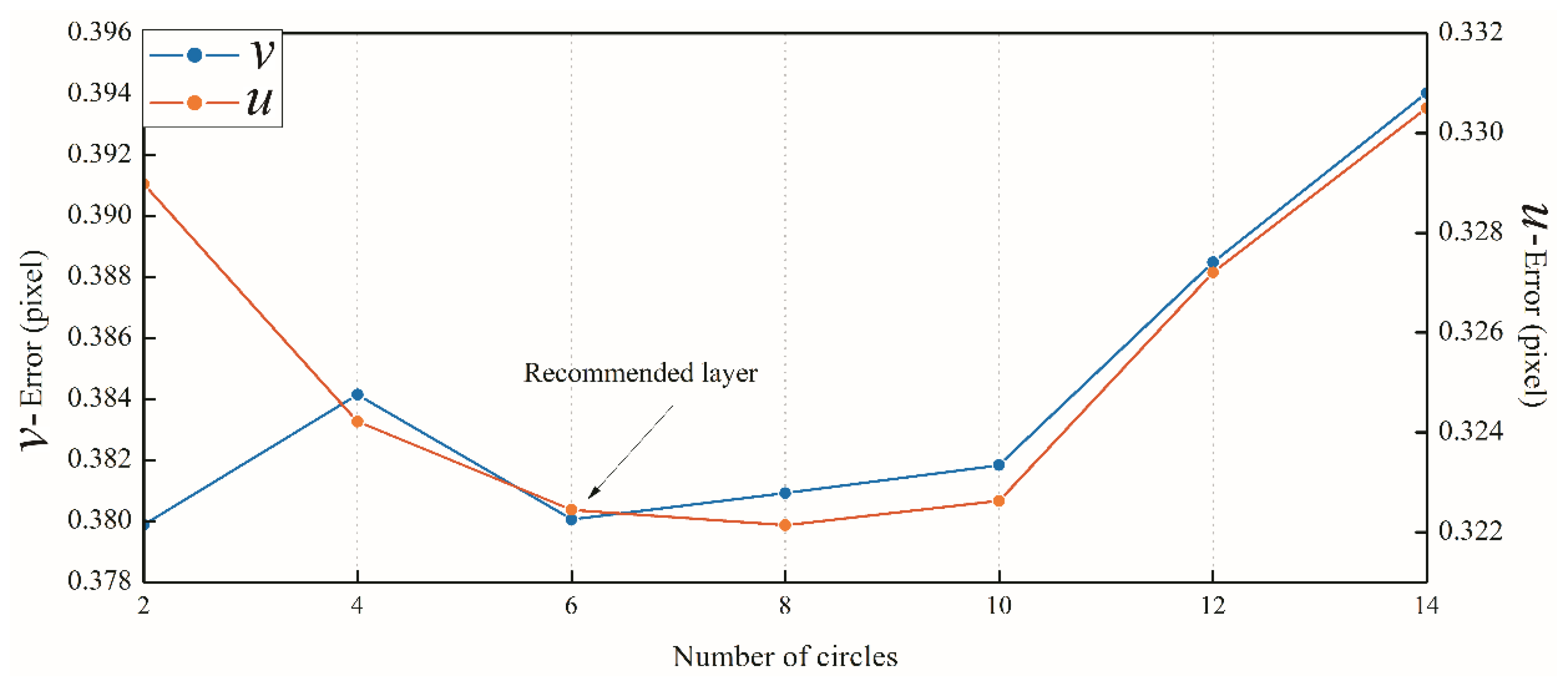
2.2.3. Target Parameter Design

(1) Number of Circles
The optimal number of concentric circles is determined based on the central location technology of the marked points described in the previous section. The test image is an idealised concentric circle of different layers with a size of 1712 × 1712 pixels, and the 2-layer concentric circles are minimal, with diameters of 10 mm and 20 mm, respectively. Then, we add circles outside the previous 2-layer concentric circles with a bigger 5 mm radius in other six patterns of concentric circles.
As shown in Table 1 and Figure 3, errors of the target coordinates generally decrease with the increase in concentric circles and then experience a relatively stable stage at layer 6 to 10. With the continuous increase in concentric circles, errors also rise almost linearly. Considering that in field measurement, when the number of concentric circles increases, the size of the targets increases accordingly, and the image noise caused by environmental factors such as air flow will also increase. To avoid this problem and save the early time cost, this study suggests setting the number of concentric layers to six (see Figure 3). At the same time, we can see that the algorithm has a deviation of 0.4 pixels. Since this deviation is stable, the center of each positioning is almost constant, so the accuracy requirements of the measurement system are met.
(2) Minimum positioning size
At different measurement distances, the pixel sizes of the targets in the image plane of the camera are inconsistent. This study will use six concentric (ellipse) circles with different pixel sizes to obtain the minimum detectable pixel size through the above-mentioned centring location technique, and thus provide guidance for a slope monitoring landmark design.
From the positioning error analysis results (see Table 2), the positioning point is located on the upper-left side of the theoretical point when the pixel resolution is above 28 × 28 pixels. The positioning error u is between 0.34 and 0.42, and the floating range is 0.07 pixels. Meanwhile, the positioning error ν is between 0.25 and 0.40, and the floating range is 0.25 pixels. It can be seen that the center of its positioning is relatively stable. In summary, this study suggests that the concentric pixel resolution should be greater than 28 × 28 pixels to ensure its effective positioning.

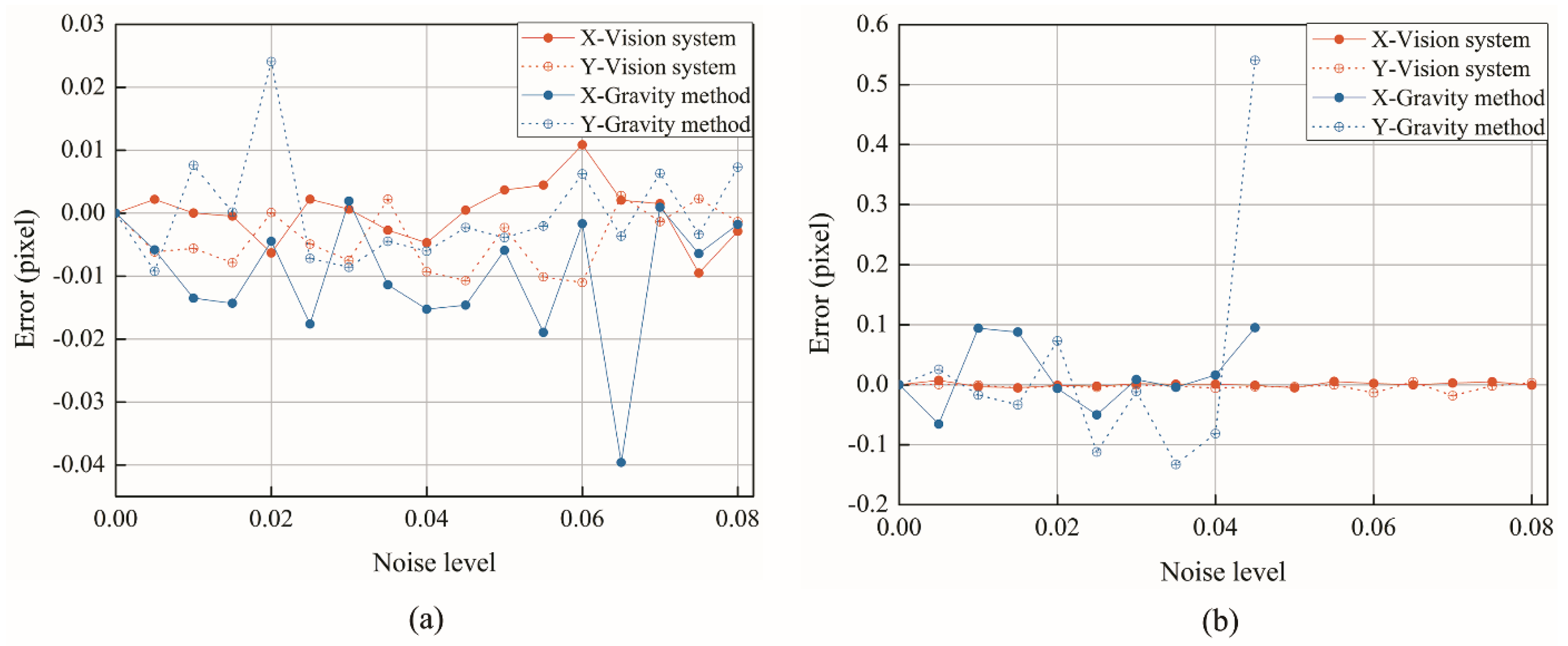
2.2.4. Noise Robustness

In image processing, noise is a ubiquitous phenomenon with great interference. In engineering applications, the obtained image is different from the “real” image due to the factors such as image acquisition equipment and natural environment. This part of difference is noise. In this section, the simulation noise image is used to verify the stability of the algorithm. At present, the image noise is mainly gaussian noise and salt noise.
In this study, the 6-layer concentric circle images, a size of 767 × 767 pixels, with different variance Gaussian noise and different density impulse noise were obtained by means of Matlab simulation, and then the positioning experiment was carried out. Compared with the measured values in the non-noise case, the error of the proposed algorithm under the influence of noise is calculated. Finally, the stability of the proposed algorithm in dealing with noise is verified by comparison with the gravity method [23] based on regional positioning.
As shown in Figure 4, when we increase the two noise levels to 0.08 respectively, we can see from the error analysis results that the fluctuation of the gravity method represented by the blue curve is significantly higher than that of the red curve. Locally, the centering technique based on the gravity method has a mis-positioning point when the impulse noise density reaches 0.05, and the center positioning cannot be achieved. The algorithm proposed in this study can still achieve accurate positioning when the impulse noise density reaches 0.08, and the maximum error is only 0.0183 (see Table 3). It is proved that the concentric center positioning method proposed in this study shows better accuracy and stability when dealing with noise.

2.3. Target Tracking
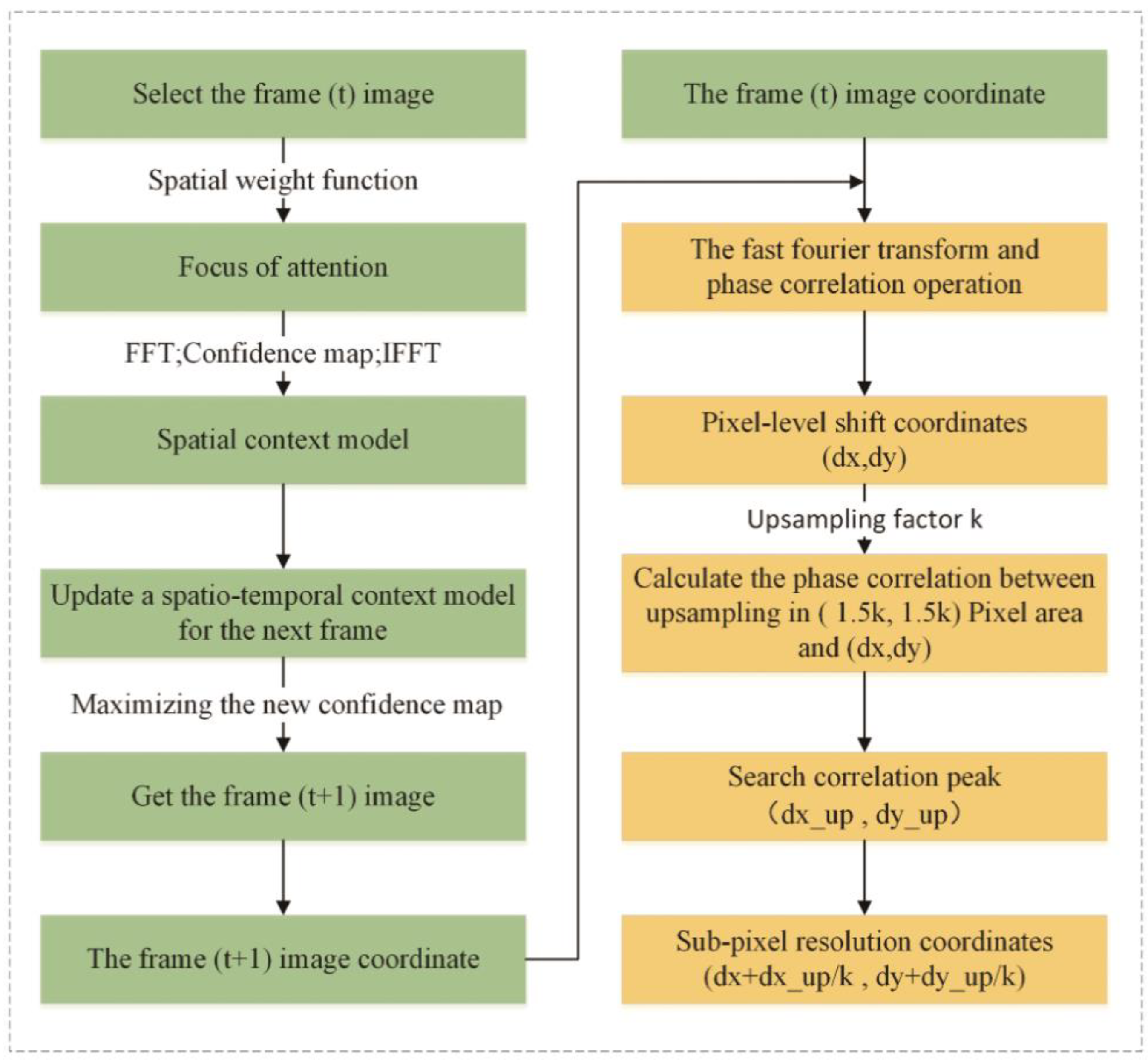
2.3.1. Theory

The STC tracking algorithm and sub-pixel image registration technology are employed to improve the target tracking accuracy. Theoretically, the accuracy of this method can probably increase to the sub-pixel level while maintaining the high speed of the STC algorithm. The basic flow is shown in Figure 5.
Step 1: Target pixel-level positioning based on a confidence map. In the first frame, we suppose that the target location has been manually initialised. At the t-th frame, we learn the spatial context model h s c ( x ) for (3) updating the spatio-temporal context model H t + 1 s t c (4) and apply it to detect the object location in the (t + 1)-th frame. The object location x t + 1 (5) in the (t + 1)-th frame is determined by maximising the new confidence map.
h s c ( x ) = F 1 ( F ( b e | x x α | β ) F ( I ( x ) ω σ ( x x ) ) )
H t + 1 s t c = ( 1 ρ ) H t s t c + ρ h t s c
x t + 1 = argmax x Ω c ( x t ) c t + 1 ( x )
where c t + 1 ( x ) is represented as
c t + 1 ( x ) = F 1 ( F ( H t + 1 s t c ( x ) ) F ( I t + 1 ( x ) ω σ t ( x x t ) ) )
In this function, F denotes the fast Fourier transform function, F 1 is the inverse of F , b is a normalisation constant, α is a scale parameter, β is a shape parameter, I ( ) is the image intensity that represents the appearance of the context, and ω σ ( ) is the weighted function defined by
ω σ ( z ) = a e | z | 2 σ 2
where a is a normalisation constant, and σ is a scale parameter.
Step 2: Target sub-pixel-level location based on image registration. UCC template matching technology is used to conduct template matching between the target and template images. The cross-correlation in the neighbourhood of 1.5 × 1.5 pixels with respect to the initial estimate is calculated using the up-sampling factor k, which can achieve a 1/k registration accuracy of the pixel, eliminate the tracking drift, and allow the tracking process to reach the sub-pixel accuracy. The specific process is as follows:
We assume that the t-frame target tracking image is f ( x , y ) , template image is g ( x , y ) , and the amount of drift between the two images is ( d x , d y ) .
g ( x , y ) = f ( x d x , y d y )
Convert the image into frequency domain using Fourier transforms:
G ( u , v ) = F ( u , v ) e i 2 π ( u d x + v d y )
Divide the above equation to obtain the cross power spectrum:
H ( u , v ) = G ( u , v ) F ( u , v ) | G ( u , v ) | | F ( u , v ) | = e i 2 π ( u d x + v d y )
In this function, F represents the complex conjugate of F . For the mutual power spectrum, the Dirac function can be obtained by inverse Fourier transform. The pixel-level registration is finally achieved by locating the peak coordinates of the Dirac function.
After achieving pixel-level registration, the pixel-level drift value of the image can be obtained, and then the sub-pixel drift coordinate extraction is implemented by using the upsampling algorithm within one pixel drift. The upsampling multiple k = 100, therefore, the registration accuracy can reach 0.01. After the image is amplified by upsampling, the image phase correlation algorithm is used to obtain the drift value of the image. Since the image drift value at this time is the result after the upsampling, it is necessary to perform the reduction in combination with the upsampling multiple, that is, multiply by 0.01 to obtain the sub-pixel drift coordinates. After obtaining the pixel-level and sub-pixel translation coordinates respectively, the final result of sub-pixel image registration can be obtained by combining the two.
In this study, the above-mentioned upsampling and image phase correlation algorithm is used to correct the drift phenomenon of the target tracking process, and then the tracking coordinates can be combined to achieve accurate target positioning. Eventually the target tracking accuracy is raised to the sub-pixel level.

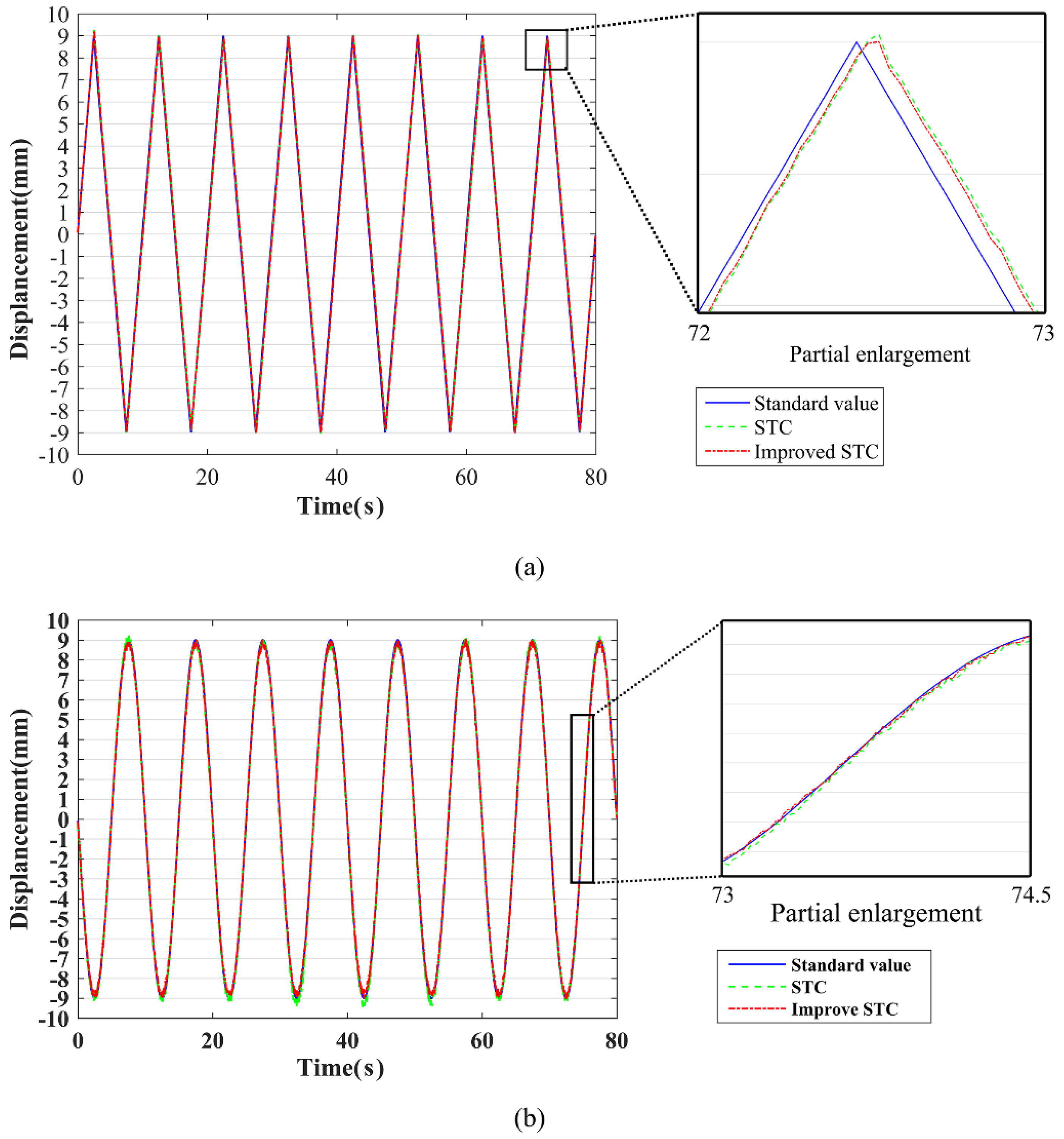
2.3.2. Performance Evaluation

The moving platform test experiments were used to evaluate the performance of the improved STC algorithm. In this study, the MTS test machine was used to clamp the moving plate to reciprocate up and down, and it was continuously monitored by the camera. In order to better demonstrate the advantages of the improved STC algorithm, two different loading methods were set up in this study, namely linear loading and sinusoidal loading. The frequency of the MTS tester was set to 0.1 Hz and the amplitude was set to 9 mm. The moving platform test setup is shown in Figure 6.
After obtaining the moving plate test sequence image, the target object is tracked and detected by using the STC algorithm and the improved STC algorithm. The pixel coordinate transformation is converted into physical coordinate transformation by the scale factor calculation method [41], and the result is shown in Figure 7.
As shown in Figure 7, both the STC algorithm and the improved STC algorithm can achieve target tracking measurements. From the partial enlargement, the measured value of the improved STC algorithm is less fluctuating. According to the measurement error analysis, the normalized root mean squared error (NRMSE) of the STC algorithm is 0.0127 for linear loading, and the improved STC algorithm is 0.0106. When sinusoidal loading, NRMSE of the STC algorithm measurement is 0.0122, and the improved STC algorithm is 0.0098. It can be seen that the improved STC algorithm can effectively reduce the measurement error, improve the measurement accuracy, and make the measurement result more stable and reliable.

2.4. Coordinate Transformation

According to Zhang’s calibration method [42], two coefficient matrices can be constructed by calibrating a binocular camera. The left- and right-image pixel coordinates are then combined using a coefficient matrix to solve the over-determined equations and obtain the spatial coordinates. After obtaining the spatial coordinates of the target in each frame of the image, the displacement value of the measurement point can be quantified to obtain the surface deformation of the slope. The calculation principle is shown in Figure 8.
[ u 1 v 1 1 ] = [ p 00 1 p 01 1 p 02 1 p 03 1 p 10 1 p 11 1 p 12 1 p 13 1 p 20 1 p 21 1 p 22 1 p 23 1 ] [ X Y Z 1 ] [ u 2 v 2 1 ] = [ p 00 2 p 01 2 p 02 2 p 03 2 p 10 2 p 11 2 p 12 2 p 13 2 p 20 2 p 21 2 p 22 2 p 23 2 ] [ X Y Z 1 ]

3. In-Laboratory Validation Test

This chapter describes tests to verify the method proposed in this study.

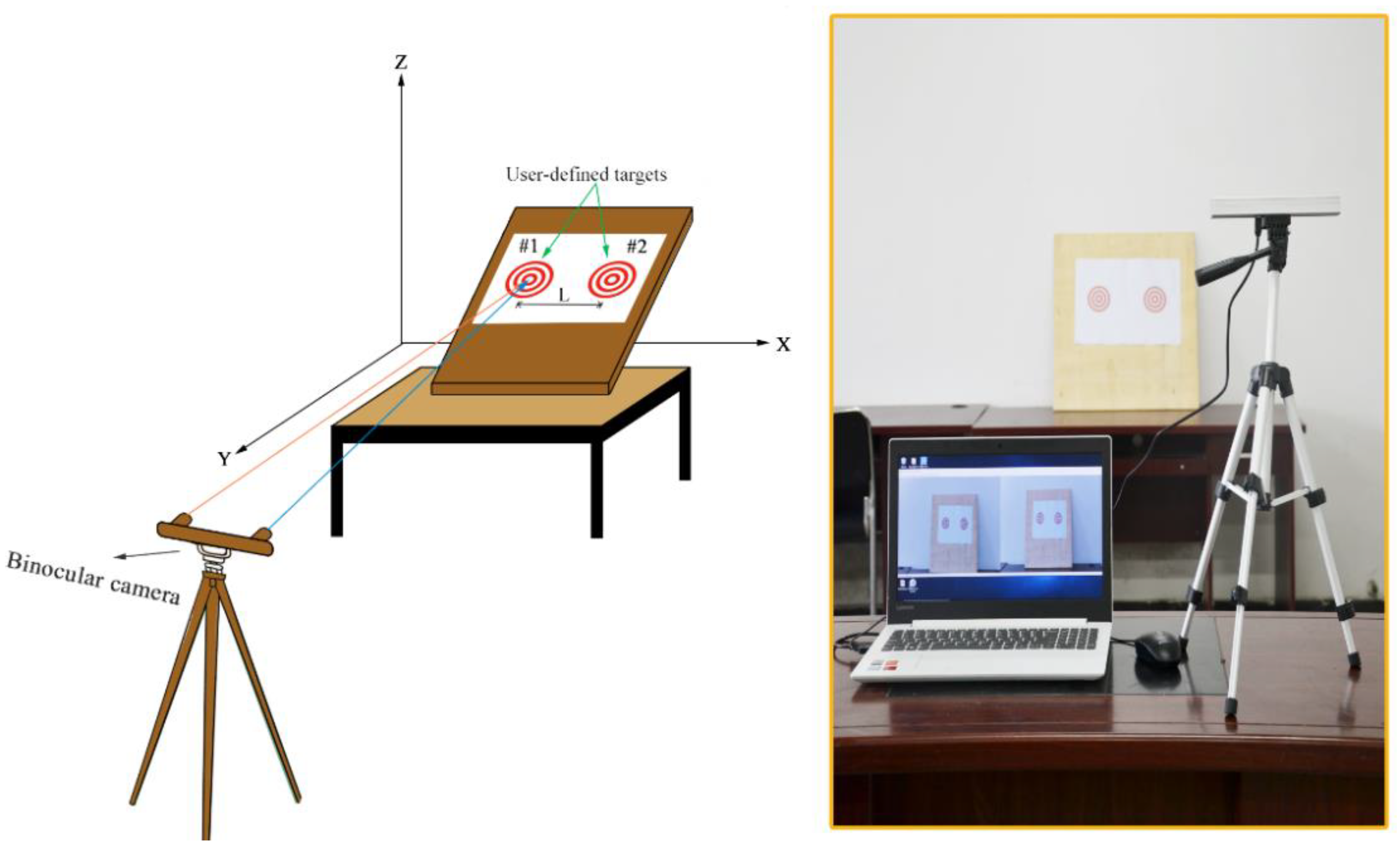
3.1. Static Distance Measurement Test

To quantify the effect of the mark point size and centre distance on the measurement accuracy, two sets of tests are described in this section. The major instrumentation includes the targets, binocular cameras, and computer (see Figure 9). The stereo baseline is set to 12 cm, and the distance from the camera to the measuring point is 4 m. Then, we get the best image by manually adjusting the focus and keep it constant.
Test 1: The sizes of the marked points are different, and the centres of the circles are the same. The marker points were designed using eight different sizes according to the relevant parameters in Chapter 3. It is assumed that the minimum concentric diameter is D , the remaining diameters are D n = D × n , n is an integer from 1 to 6, and the distance between two centres is 150 mm accordingly, which is measured in vector drawing tool Coreldraw.
Test 2: The marked points have the same size, but the centres of the two circles are different. We chose a minimum diameter of the marker point of 15 mm, and a distance to the circle centre of 100 to 300 mm.
The results obtained after calculating the spatial coordinates using the proposed method in Chapter 2 are shown in Table 4 and Table 5.
As can be seen from the above table, during the testing of different target size measurements, the distance between the two markers was measured using a stereo-vision system. The mean value of the measurement error is 0.1923 mm, and the maximum error is 0.2367 mm. During the testing of the circle centre distance for different sign points, the average value of the measurement error is 0.2153 mm, and the maximum error is 0.2898 mm. This shows that the system can achieve millimetre level accuracy in monitoring, and ensure the accuracy of the spatial coordinate measurements. Furthermore, the development of its error has no obvious relationship with the marked point size and the distance from the centre of the circle, and thus can reach the millimetre level in any sized measurement of the mark.

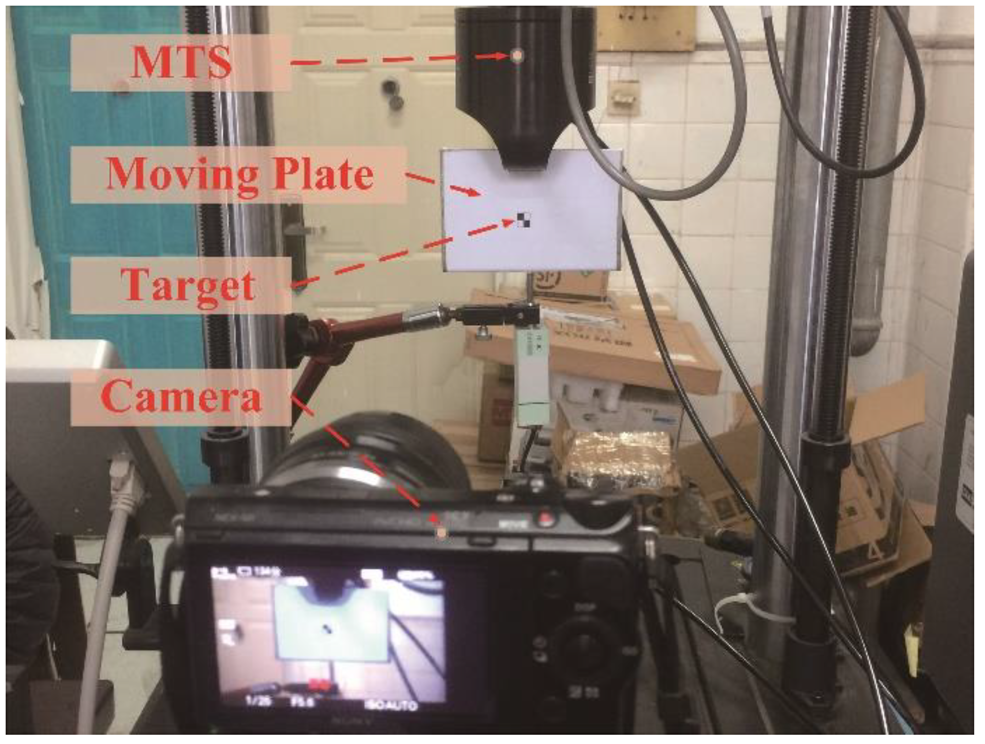
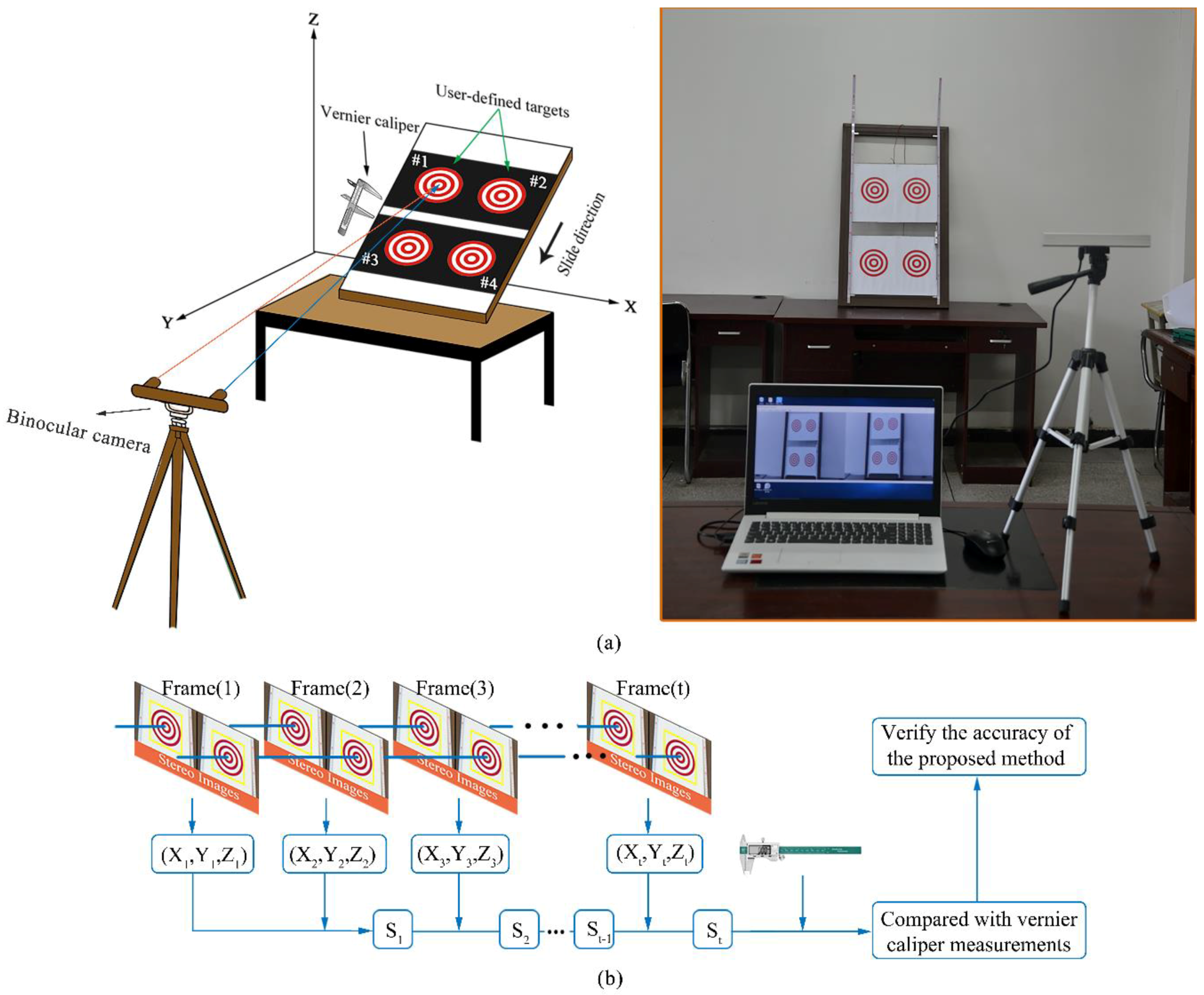
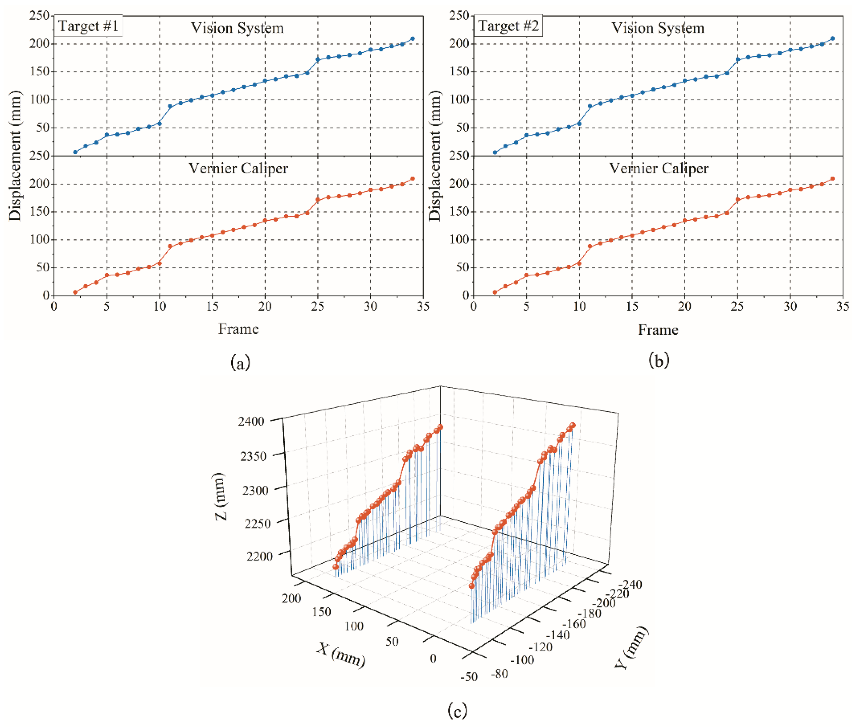
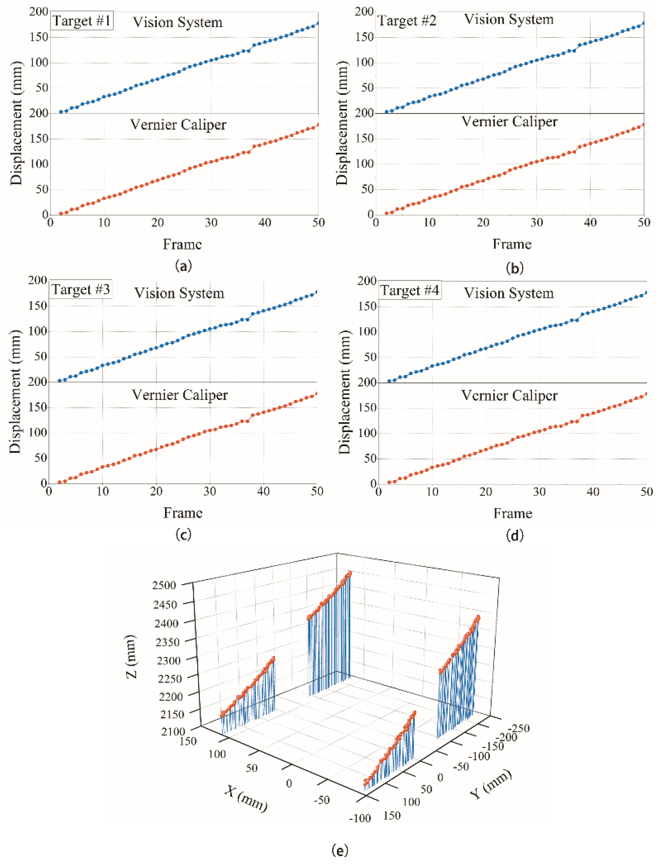
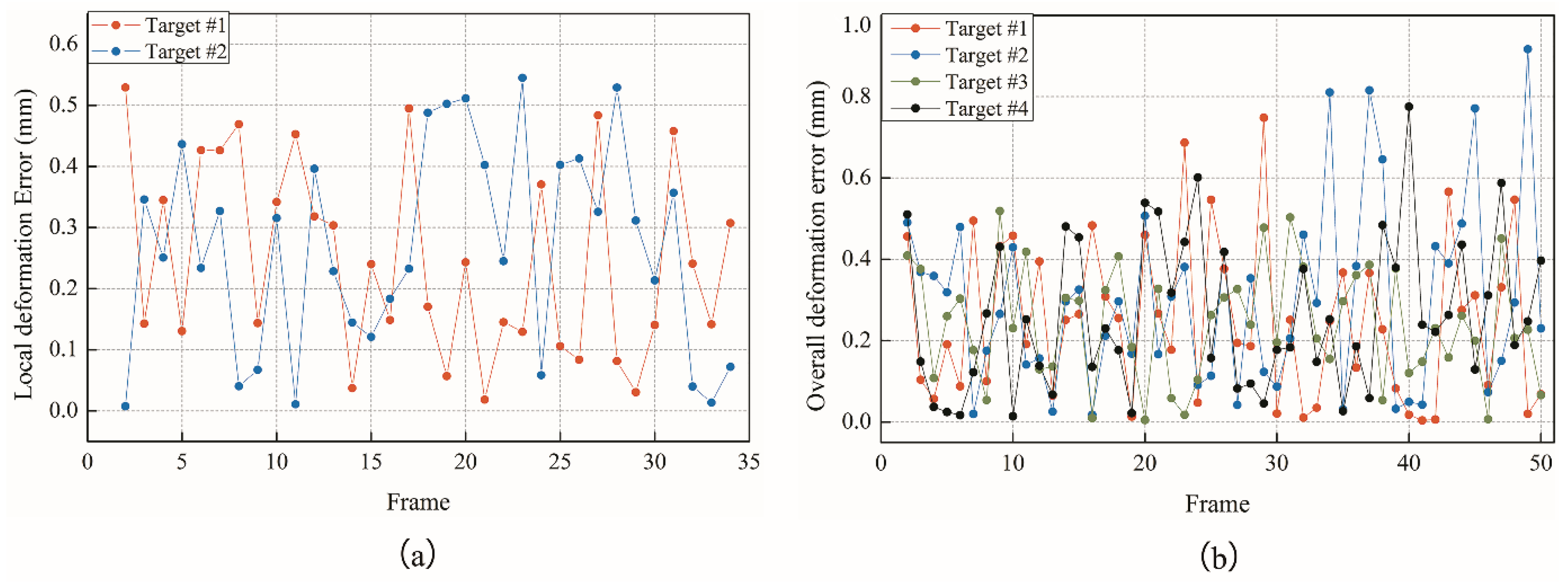
3.2. Moving Platform Experiment

The above distance measurement test verifies the accuracy of the system proposed in this paper. However, the test capture process is static and cannot be used to verify the feasibility of the system. Based on this research, the laboratory model test is used to verify the tracking and positioning accuracy of the system. The overall layout of the test is shown in Figure 10. The test instruments included slidable panels, binocular cameras, Vernier callipers, and laptops. The slidable squad consists of two plates that can slide up and down, and can simulate the local deformation and overall deformation, respectively. To compare and analyse the accuracy, the sliding distance is obtained using the binocular stereo-vision system and Vernier calliper, respectively.
Test 1: Local deformation monitoring test. The lower plate is fixed in the sliding plate group, and the upper plate is moved slowly downwards. At the same time, a Vernier calliper and a binocular stereo-vision system are used to measure the distance between the two objects in the upper plate. A total of 34 frames are tested.
Test 2: Overall deformation monitoring test. The slope deformation is simulated by connecting the upper and lower plates, and moving them slowly at the same time. The displacement is quantified by monitoring the changes in the spatial position of the four landmarks.
The test results obtained are shown in Figure 11, Figure 12 and Figure 13.
It can be seen from the above test data that the spatial displacement value tracked by the binocular stereo-vision measurement system is compared with the displacement value measured using the Vernier calliper. Through local deformation monitoring error can be obtained (see Figure 11 and Figure 13a), The average value of the error is 0.2568 mm, and the maximum error is 0.5427 mm. Only five of the 68 groups of measurement data have errors exceeding 0.5 mm, which proves that the binocular stereo-vision measurement system has strong tracking and positioning stability. The results of the overall deformation-monitoring test are shown in Figure 12 and Figure 13b. The average values of the monitoring errors for each marker are 0.2503, 0.2995, 0.2404, and 0.2619 mm, respectively, and the maximum error is 0.9219 mm. In the two hundred groups of stereo-vision system measurements, there are three groups with errors exceeding 0.8 mm, six groups with errors exceeding 0.7 mm, and eight groups with errors exceeding 0.6 mm. In addition, the mean and maximum values of the error are increased relative to the static measurement test. This is because there is a certain error in the target-tracking process, which causes the average error and fluctuation range to increase.

4. Conclusions

The exploration of structural health monitoring based on vision sensors is still in its infancy. In this study, a non-contact dynamic displacement measurement system with binocular stereo vision is designed. The slope is used as a carrier to explore the possibility of tracking and positioning technology to monitor the three-dimensional deformation of the structure. The specific conclusions are as follows:
(1)
Target markers adapted to the monitoring system are specially designed as concentric circles. Considering the error of program operation, graphics positioning size and time cost, the research suggests setting the number of concentric layers to six, and the pixel size of the marker points to no smaller than 28 × 28 pixels. Under the design of the target, it can be seen from the noise robustness test that the positioning method has better positioning accuracy and stability under different levels of Gaussian noise and impulse noise than the center of gravity method.
(2)
This study successfully introduces the target tracking technology into the deformation monitoring of the slope and improves the degree of intelligence. The tracking performance evaluation test shows that the use of UCC sub-pixel template matching technology to optimize the tracking accuracy of an STC target can effectively reduce the measurement error.
(3)
Finally, slope movement is simulated by the indoor sliding plate, and the deformation is monitored employing the proposed method. The results show that the accuracy of the deformation measurement can achieve a millimeter level. It validates the potentials of the stereo vision displacement sensor for cost-effective slope health monitoring. However, the actual slope application needs to be further explored according to the actual situation.
The vision sensor system proposed in this paper can also be applied to deformation monitoring scenarios in other engineering fields, such as bridge deflection, tunnel convergence, and also structural deformation. However, detailed monitoring plans in these circumstances should take into full consideration specific site conditions and the primary monitoring objects closely related to the structural health.

Author Contributions

The asterisk indicates the corresponding author, and the first two authors contributed equally to this work. The vision sensor system is developed by J.T. and S.H., under the supervision of Q.H. and L.H. Experiment planning, setup and measurement of laboratory tests are conducted by Q.C., Y.F., S.T. provided valuable insight in preparing this manuscript.

Funding

This research was funded by the National Natural Science Foundation of China (Grant No. 51574201) and the Scientific and Technical Youth Innovation Group (Southwest Petroleum University) (2015CXTD05).

Conflicts of Interest

The authors declare no conflict of interest.

References

  1. Marek, L.; Miřijovský, J.; Tuček, P. Monitoring of the Shallow Landslide Using UAV Photogrammetry and Geodetic Measurements. In Engineering Geology for Society and Territory; Springer: Berlin, Germany, 2015; Volume 2, pp. 113–116. [Google Scholar]
  2. Benoit, L.; Briole, P.; Martin, O.; Thom, C.; Malet, J.P.; Ulrich, P. Monitoring landslide displacements with the Geocube wireless network of low-cost GPS. Eng. Geol. 2015, 195, 111–121. [Google Scholar] [CrossRef]
  3. China National Standards. GB 50026-2007, Code for Engineering Surveying; China Planning Press: Shenzhen, China, 2008; p. 8.
  4. Abellán, A.; Oppikofer, T.; Jaboyedoff, M.; Rosser, N.J.; Lim, M.; Lato, M.J. Terrestrial laser scanning of rock slope instabilities. Earth Surf. Process. Landf. 2014, 39, 80–97. [Google Scholar] [CrossRef]
  5. Sun, Q.; Zhang, L.; Ding, X.L.; Hu, J.; Li, Z.W.; Zhu, J.J. Slope deformation prior to Zhouqu, China landslide from InSAR time series analysis. Remote Sens. Environ. 2015, 156, 45–57. [Google Scholar] [CrossRef]
  6. Feng, D.; Feng, M.Q.; Ozer, E.; Fukuda, Y. A Vision-Based Sensor for Noncontact Structural Displacement Measurement. Sensors 2015, 15, 16557–16575. [Google Scholar] [CrossRef] [PubMed] [Green Version]
  7. Yoon, H.; Elanwar, H.; Choi, H.; Golparvar-Fard, M.; Spencer, B.F. Target-free approach for vision-based structural system identification using consumer-grade cameras. Struct. Control Health Monit. 2016, 23, 1405–1416. [Google Scholar] [CrossRef]
  8. Khuc, T.; Catbas, F.N. Completely contactless structural health monitoring of real-life structures using cameras and computer vision. J. Int. Assoc. Struct. Control Monit. 2017, 24. [Google Scholar] [CrossRef]
  9. Harris, C.; Stephens, M. A Combined Corner and Edge Detector. Proc. Alvey Vis. Conf. 1988, 1988, 147–151. [Google Scholar]
  10. Bay, H.; Ess, A.; Tuytelaars, T.; Gool, L.V. Speeded-Up Robust Features (SURF). Comput. Vis. Image Understand. 2008, 110, 346–359. [Google Scholar] [CrossRef] [Green Version]
  11. Chang, C.C.; Ji, Y.F. Flexible Videogrammetric Technique for Three-Dimensional Structural Vibration Measurement. J. Eng. Mech. 2007, 133, 656–664. [Google Scholar] [CrossRef]
  12. Choi, I.; Kim, J.; Kim, D. A Target-Less Vision-Based Displacement Sensor Based on Image Convex Hull Optimization for Measuring the Dynamic Response of Building Structures. Sensors 2016, 16, 2085. [Google Scholar] [CrossRef] [PubMed]
  13. Hu, Q.; He, S.; Wang, S.; Liu, Y.; Zhang, Z.; He, L.; Wang, F.; Cai, Q.; Shi, R.; Yang, Y. A High-Speed Target-Free Vision-Based Sensor for Bus Rapid Transit Viaduct Vibration Measurements Using CMT and ORB Algorithms. Sensors 2017, 17, 1305. [Google Scholar] [CrossRef] [PubMed]
  14. Feng, D.; Feng, M.Q. Experimental validation of cost-effective vision-based structural health monitoring. Mech. Syst. Signal Process. 2017, 88, 199–211. [Google Scholar] [CrossRef]
  15. Choi, H.S.; Cheung, J.H.; Kim, S.H.; Ahn, J.H. Structural dynamic displacement vision system using digital image processing. NDT E Int. 2011, 44, 597–608. [Google Scholar] [CrossRef]
  16. Song, Y.Z.; Bowen, C.R.; Kim, A.H.; Nassehi, A.; Padget, J.; Gathercole, N. Virtual visual sensors and their application in structural health monitoring. Struct. Health Monit. 2014, 13, 251–264. [Google Scholar] [CrossRef] [Green Version]
  17. Zhao, X.; Liu, H.; Yu, Y.; Xu, X.; Hu, W.; Li, M.; Ou, J. Bridge displacement monitoring method based on laser projection-sensing technology. Sensors 2015, 15, 8444–8463. [Google Scholar] [CrossRef] [PubMed]
  18. Jeon, H.; Kim, Y.; Lee, D.; Myung, H. Vision-Based Remote 6-DOF Structural Displacement Monitoring System Using a Unique Marker. Smart Struct. Syst. 2014, 13, 927–942. [Google Scholar] [CrossRef]
  19. Shariati, A.; Schumacher, T. Eulerian-based virtual visual sensors to measure dynamic displacements of structures. Struct. Control Health Monit. 2017, 24, e1977. [Google Scholar] [CrossRef]
  20. Feng, D.; Feng, M.Q. Vision-based multipoint displacement measurement for structural health monitoring. Struct. Control Health Monit. 2016, 23, 876–890. [Google Scholar] [CrossRef]
  21. Ye, X.W.; Yi, T.H.; Dong, C.Z.; Liu, T. Vision-based structural displacement measurement: System performance evaluation and influence factor analysis. Measurement 2016, 88, 372–384. [Google Scholar] [CrossRef]
  22. Lee, H.; Rhee, H.; Oh, J.H.; Jin, H.P. Measurement of 3-D Vibrational Motion by Dynamic Photogrammetry Using Least-Square Image Matching for Sub-Pixel Targeting to Improve Accuracy. Sensors 2016, 16, 359. [Google Scholar] [CrossRef] [PubMed]
  23. Xu, W.; Li, Q.; Feng, H.J.; Xu, Z.H.; Chen, Y.T. A novel star image thresholding method for effective segmentation and centroid statistics. Optik Int. J. Light Electron Opt. 2013, 124, 4673–4677. [Google Scholar] [CrossRef]
  24. Weng, M.; He, M. Image detection based on SUSAN method and integrated feature matching. Int. J. Innov. Comput. Inf. Control Ijicic 2008, 4, 671–680. [Google Scholar]
  25. Hollitt, C. A convolution approach to the circle Hough transform for arbitrary radius. Mach. Vis. Appl. 2013, 24, 683–694. [Google Scholar] [CrossRef]
  26. Shi, J.; Tomasi, C. Good features to track. In Proceedings of the IEEE Conference on Computer Vision and Pattern Recognition (CVPR’94), Seattle, WA, USA, 21–23 June 1994. [Google Scholar]
  27. Danelljan, M.; Khan, F.S.; Felsberg, M.; Weijer, J.V.D. Adaptive Color Attributes for Real-Time Visual Tracking. In Proceedings of the IEEE Conference on Computer Vision and Pattern Recognition, Beijing, China, 23–28 June 2014; pp. 1090–1097. [Google Scholar]
  28. Henriques, J.F.; Rui, C.; Martins, P.; Batista, J. High-Speed Tracking with Kernelized Correlation Filters. IEEE Trans. Pattern Anal. Mach. Intell. 2015, 37, 583–596. [Google Scholar] [CrossRef] [PubMed] [Green Version]
  29. Zhang, K.; Zhang, L.; Yang, M.H. Real-time object tracking via online discriminative feature selection. IEEE Trans. Image Process. 2013, 22, 4664–4677. [Google Scholar] [CrossRef] [PubMed]
  30. Zhang, K.; Zhang, L.; Liu, Q.; Zhang, D.; Yang, M.H. Fast Visual Tracking via Dense Spatio-temporal Context Learning. In Proceedings of the 13th European Conference on Computer vision (ECCV), Zurich, Switzerland, 6–12 September 2014; Volume 8693, pp. 127–141. [Google Scholar]
  31. Zhang, K.; Zhang, L.; Yang, M.H.; Zhang, D. Fast Tracking via Spatio-Temporal Context Learning. arXiv, 2013; arXiv:1311.1939. [Google Scholar]
  32. Molinaviedma, A.J.; Felipesesé, L.; Lópezalba, E.; Díaz, F. High frequency mode shapes characterisation using Digital Image Correlation and phase-based motion magnification. Mech. Syst. Signal Process. 2018, 102, 245–261. [Google Scholar] [CrossRef]
  33. Javh, J.; Slavič, J.; Boltežar, M. High frequency modal identification on noisy high-speed camera data. Mech. Syst. Signal Process. 2018, 98, 344–351. [Google Scholar] [CrossRef]
  34. Javh, J.; Slavič, J.; Boltežar, M. The subpixel resolution of optical-flow-based modal analysis. Mech. Syst. Signal Process. 2017, 88, 89–99. [Google Scholar] [CrossRef]
  35. Xu, Y.; Brownjohn, J.; Kong, D. A non-contact vision-based system for multipoint displacement monitoring in a cable-stayed footbridge. Struct. Control Health Monit. 2018, 25, e2155. [Google Scholar] [CrossRef] [Green Version]
  36. Guizar-Sicairos, M.; Thurman, S.T.; Fienup, J.R. Efficient subpixel image registration algorithms. Opt. Lett. 2008, 33, 156. [Google Scholar] [CrossRef] [PubMed]
  37. Zhang, G. Vision Measurement; Science Press: Beijing, China, 2008; pp. 144–148. (In Chinese) [Google Scholar]
  38. Gao, S.Y. Improved Algorithm about Subpixel Edge Detection of Image Based on Zernike Orthogonal Moments. Acta Autom. Sin. 2008, 34, 1163–1168. [Google Scholar] [CrossRef]
  39. Gander, W.; Golub, G.H.; Strebel, R. Least-Squares Fitting of Circles and Ellipses. BIT Numer. Math. 1994, 34, 558–578. [Google Scholar] [CrossRef]
  40. Zhang, H.; Yu, H.; Li, Y.; Hu, B. Improved K-means Algorithm Based on the Clustering Reliability Analysis. In Proceedings of the International Symposium on Computers and Informatics, Beijing, China, 17–18 January 2015. [Google Scholar]
  41. Sun, S.-G.; Wang, C.; Zhao, J.; Destech Publicat, I. The Application of Improved GM (1,1) Model in Deformation Prediction of Slope. In Proceedings of the 2nd International Conference on Sustainable Energy and Environmental Engineering, Xiamen, China, 18–19 December 2016. [Google Scholar]
  42. Zhang, Z. A Flexible New Technique for Camera Calibration; IEEE Computer Society: Washington, DC, USA, 2000; pp. 1330–1334. [Google Scholar]
Figure 1. Displacement measurement system based on binocular vision technology: (a) hardware and (b) software.
Sensors 18 02890 g001
Figure 2. Target location process.
Sensors 18 02890 g002
Figure 3. Analysis of test results of concentric circles.
Sensors 18 02890 g003
Figure 4. Positioning error of marker points under the influence of noise; (a) Considering Gaussian noise; (b) Considering impulse noise.
Sensors 18 02890 g004
Figure 5. Flowchart of object tracking based on spatial-temporal contextual (STC) and Unsampled Cross Correlation (UCC).
Sensors 18 02890 g005
Figure 6. Setup for moving platform tests.
Sensors 18 02890 g006
Figure 7. The moving platform tests results: (a) linear loading; (b) sinusoidal loading.
Sensors 18 02890 g007
Figure 8. Schematic of binocular vision measurement.
Sensors 18 02890 g008
Figure 9. Setup for static distance measurement test, left: image of 3D simulation test, right: laboratory test scene.
Sensors 18 02890 g009
Figure 10. Moving platform experiment: (a) test site settings and (b) experimental procedure.
Sensors 18 02890 g010
Figure 11. Local deformation marker point displacement monitoring results: (a) target 1, (b) target 2, and (c) spatial results.
Sensors 18 02890 g011
Figure 12. Overall deformation marker point displacement monitoring results: (a) target 1, (b) target 2, (c) target 3, (d) target 4, and (e) spatial results.
Sensors 18 02890 g012
Figure 13. Results of measurement error: (a) Local deformation; (b) Overall deformation.
Sensors 18 02890 g013
Table 1. Error analysis of different concentric circle tests.
Number of CirclesMeasured Coordinates (pixel)True Coordinates (pixel)Error (pixel)Time
u ν u ν u ν (ms)
2855.620117855.6710218568560.3798830.3289793707
4855.615845855.6757818568560.3841550.3242193885
6855.619934855.6775518568560.3800660.3224494134
8855.619080855.6778568568560.3809200.3221444337
10855.618164855.6773688568560.3818360.3226324477
12855.611511855.6727918568560.3884890.3272094849
14855.605957855.6694958568560.3940430.3305055184
Table 2. Concentric testing of different pixel dimensions.
Size (pixels)ClassifyNumber of Circles DetectedClustering Coordinates (pixels)True Coordinates (pixels)Error (pixels)
u ν u ν u ν
41 × 41circle620.15475320.21404620.520.50.3452470.285954
ellipse620.0885320.19260620.520.50.411470.307394
36 × 36circle617.62517417.63632418180.3748260.363676
ellipse617.59489317.67311118180.4051070.326889
30 × 30circle614.61633614.70096915150.3836640.299031
ellipse614.58907614.74312315150.4109240.256877
28 × 28circle613.62541513.7223214140.3745850.27768
ellipse613.61208613.6079314140.3879140.39207
25 × 25circle513.42019711.99955112.512.5−0.92020.500449
ellipse612.43692813.60174512.512.50.063072−1.10175
Table 3. Positioning error of marker points under the influence of noise.
NumberNoise LevelGaussian Noise Error (pixels)Impulse Noise Error (pixels)
Vision SystemGravity MethodVision SystemGravity Method
u ν u ν u ν u ν
1000000000
20.0050.002198−0.00613−0.00582−0.009220.0072020.000458−0.065640.025549
30.010.000031 −0.00558−0.013490.007616−0.00336−0.000610.094164−0.01722
40.015−0.000457−0.00784−0.01430.000161−0.00513−0.005520.087803−0.0336
50.02−0.0062860.000122−0.004450.024084−0.00107−0.00293−0.006390.072873
60.0250.002228−0.00488−0.01759−0.00717−0.00241−0.00424−0.05005−0.11229
70.030.000641−0.007480.001939−0.008580.001587−0.000520.008688−0.01136
80.035−0.0026850.002228−0.01136−0.004450.000977−0.00198−0.00427−0.13275
90.04−0.004699−0.00928−0.01524−0.006030.000977−0.005980.016176−0.08148
100.0450.000489−0.01071−0.01459−0.00226−0.00095−0.003450.094990.540542
110.050.003693−0.00229−0.0059−0.00388−0.00513−0.00339
120.0550.004456−0.0101−0.01893−0.002040.005402−0.00037
130.060.010865−0.01099−0.001660.0062280.001984−0.01364
140.0650.0020760.002808−0.03957−0.00365−0.000180.004792
150.070.001526−0.001340.0009370.0063150.002747−0.01834
160.075−0.0094910.002289−0.0064−0.003340.004792−0.00192
170.08−0.002868−0.00134−0.001780.007308−0.000820.002961
Table 4. Measurement results of Test 1.
NumberMinimum DiameterPixel SizeTarget Space CoordinatesMeasurement (mm)Error (mm)
x y z
I-1566 × 66−47.249660.79721540.49149.77650.2235
101.46664.02621522.99
I-27.599 × 99−45.756648.58141526.84149.84640.1536
102.955.18741544.49
I-310132 × 132−72.031572.83571535.54150.23670.2367
76.898378.37951554.52
I-412.5165 × 165−45.52470.33831534.15149.79050.2095
101.92571.98631507.82
I-515198 × 198−33.977464.14821523.63149.83620.1638
115.167.55481538.3
I-617.5231 × 231−84.472890.95811536.39149.76840.2316
63.384591.61961512.55
I-720264 × 264−37.094687.5391517.28150.13540.1354
108.98684.46121482.76
I-822.5297 × 297−101.02685.83911518.59149.81580.1842
46.473786.61751492.36
Table 5. Measurement results of Test 2.
NumberReal (mm)Target Space CoordinatesMeasurement (mm)Error (mm)
x y z
II-1100−31.18795.20451529.29100.16810.1681
66.690295.31431507.99
II-212515.199481.91681526.35124.74680.2532
139.58185.39771535.23
II-3150−33.977464.14821523.63149.83620.1638
115.167.55481538.3
II-4175−84.989109.5881543.95174.80490.1951
87.5032109.4061515.61
II-5200−36.021565.70061538.77200.15520.1552
163.31567.54811556.76
II-6225−86.379960.43791544.6225.260.26
13761.29691573.63
II-7250−65.7222107.1951540.87250.17020.1702
183.541113.8071561.1
II-8275−52.42474.35211516.97275.28980.2898
221.94480.51411538.62
II-9300−144.00867.85411520.25300.28210.2821
154.40174.30541553.11

