A Sensor Based on a Spherical Parallel Mechanism for the Measurement of Fluid Velocity: Physical Modelling and Computational Analysis


Abstract
:1. Introduction
1.1. Motivation
1.2. Outline
2. Materials and Methods
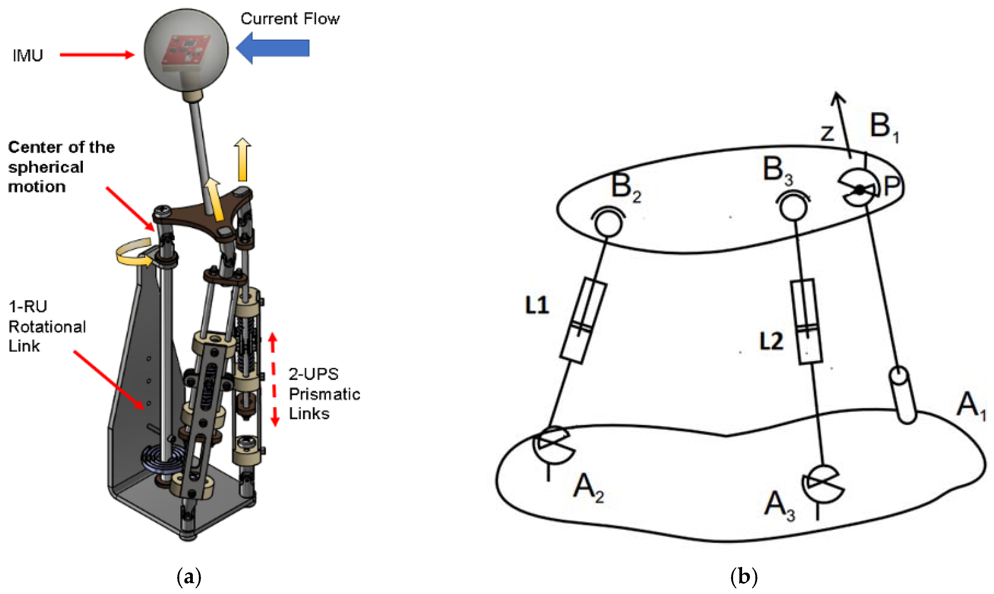
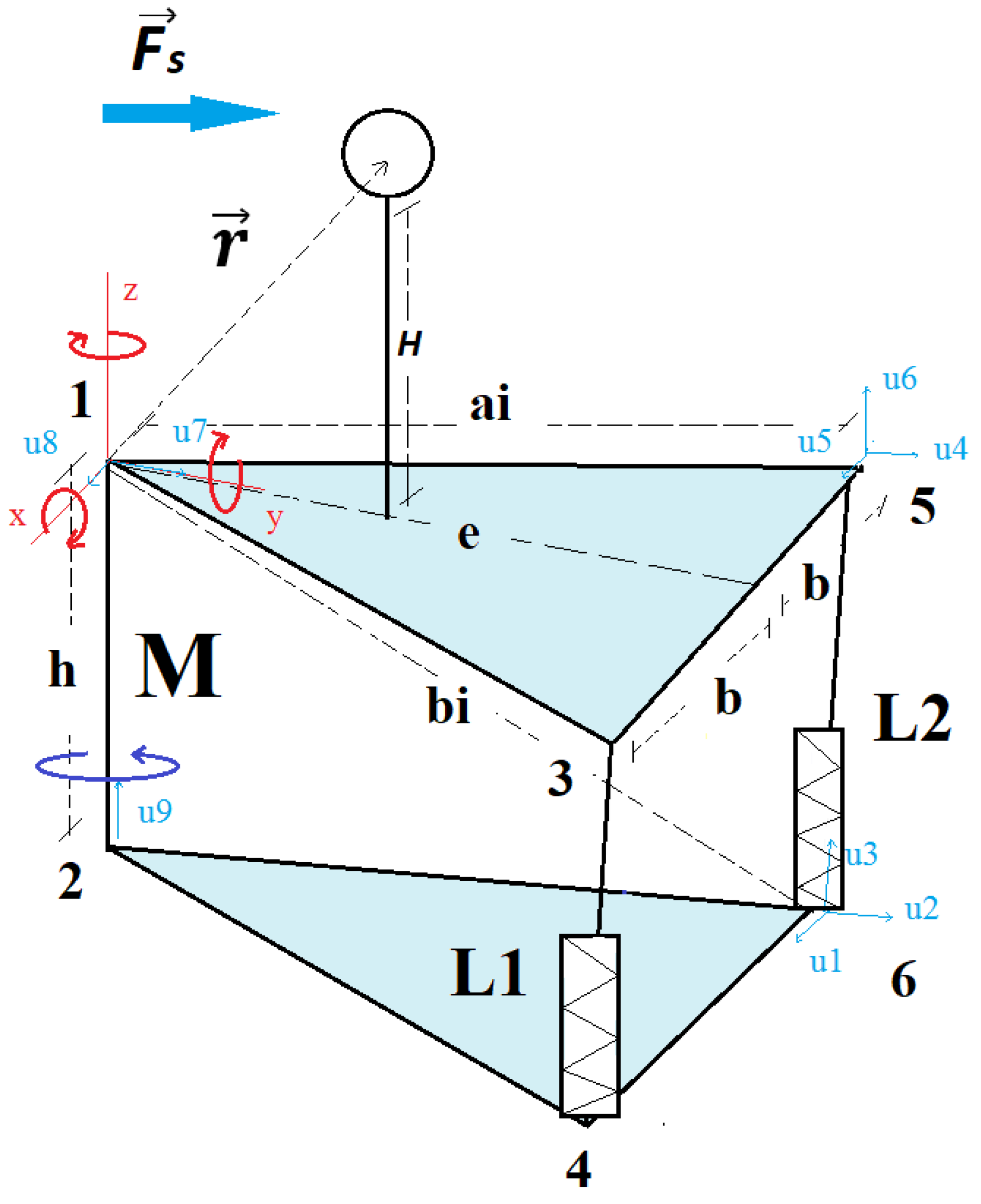
2.1. Sensor Description
2.2. Kinematics of the Parallel Mechanism
2.2.1. Calculation of the Inverse Kinematics
2.2.2. Calculation of the Jacobian Matrix
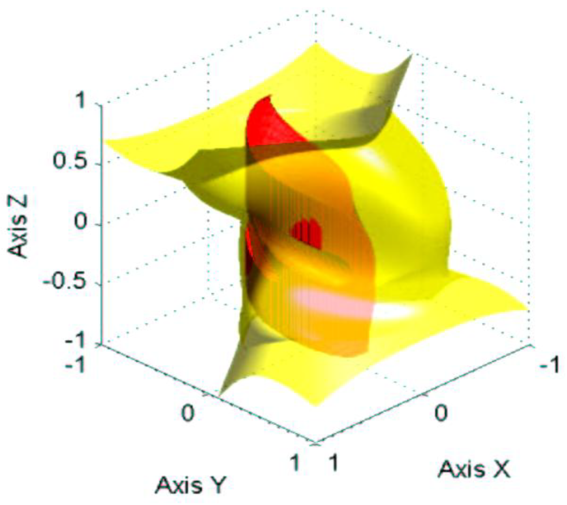
2.2.3. Analysis of Workspace and Singularities of the Parallel Mechanism
2.3. Dynamics
2.3.1. Resulting Force of Each Body Due to Buoyancy
2.3.2. Matrix of Forces and Torques of Each Actuator
2.3.3. Platform of the Parallel Mechanism
2.3.4. Cylinder of Linear Actuator i
2.3.5. Piston of the Linear Actuator i
2.3.6. Rotating Actuator
2.3.7. Velocities and Angular Accelerations
2.3.8. Jacobian Matrix of Each Actuator
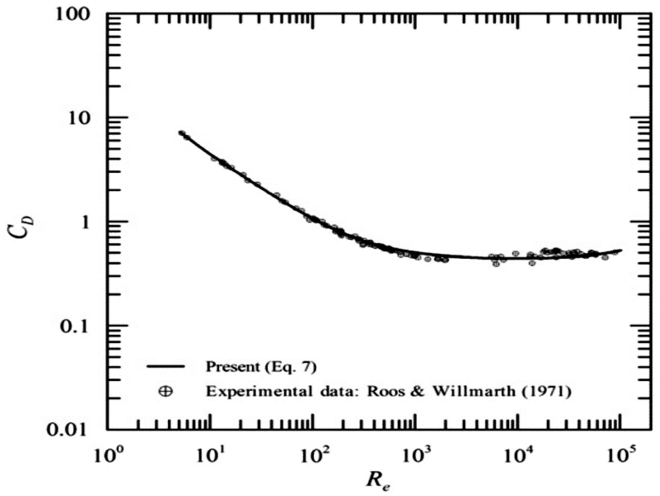
2.3.9. Torque Generated by Fluid Dynamic Forces in the Sphere
2.3.10. Velocity and Direction of the Fluid
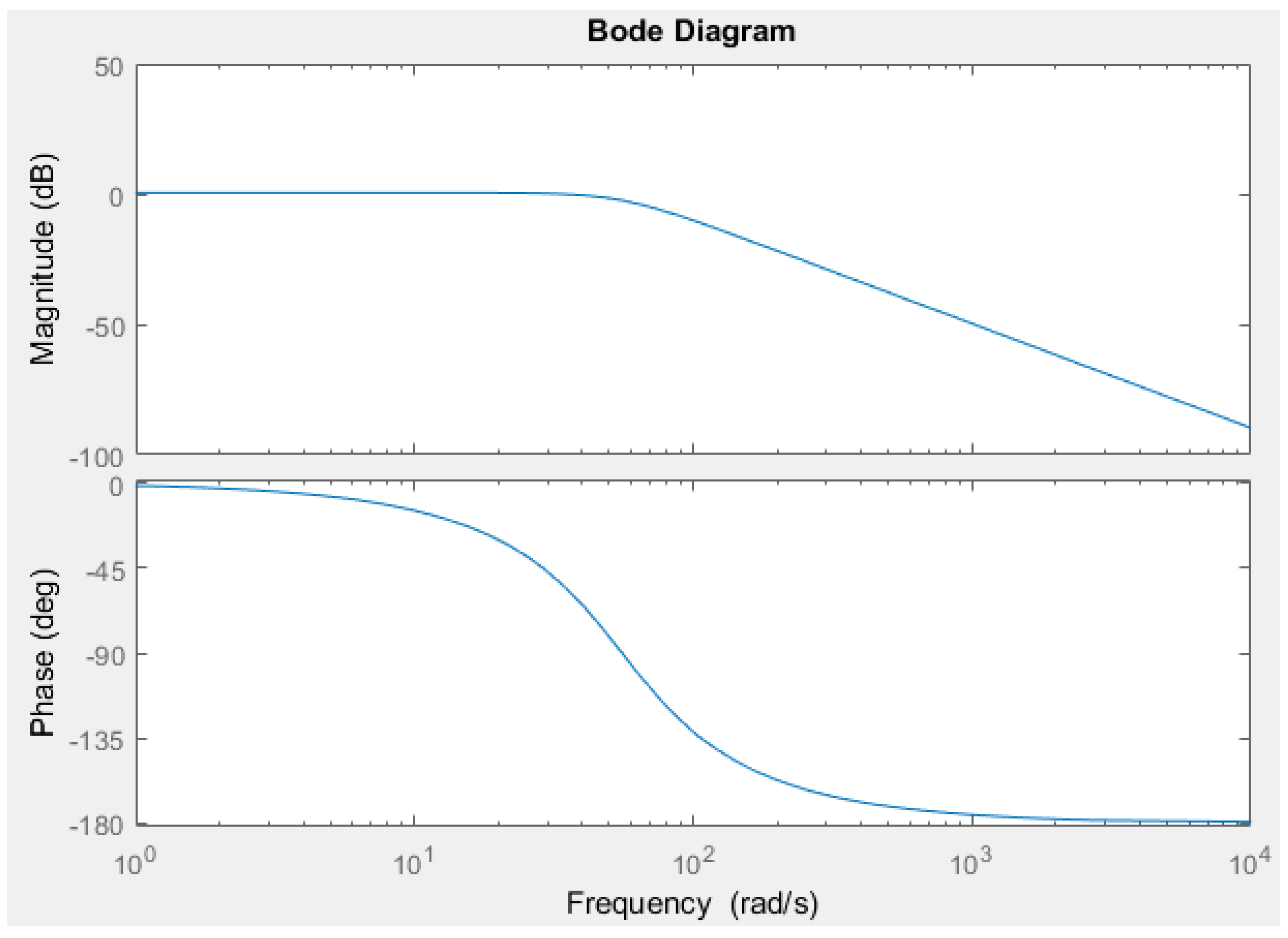
2.3.11. Dynamic Performance
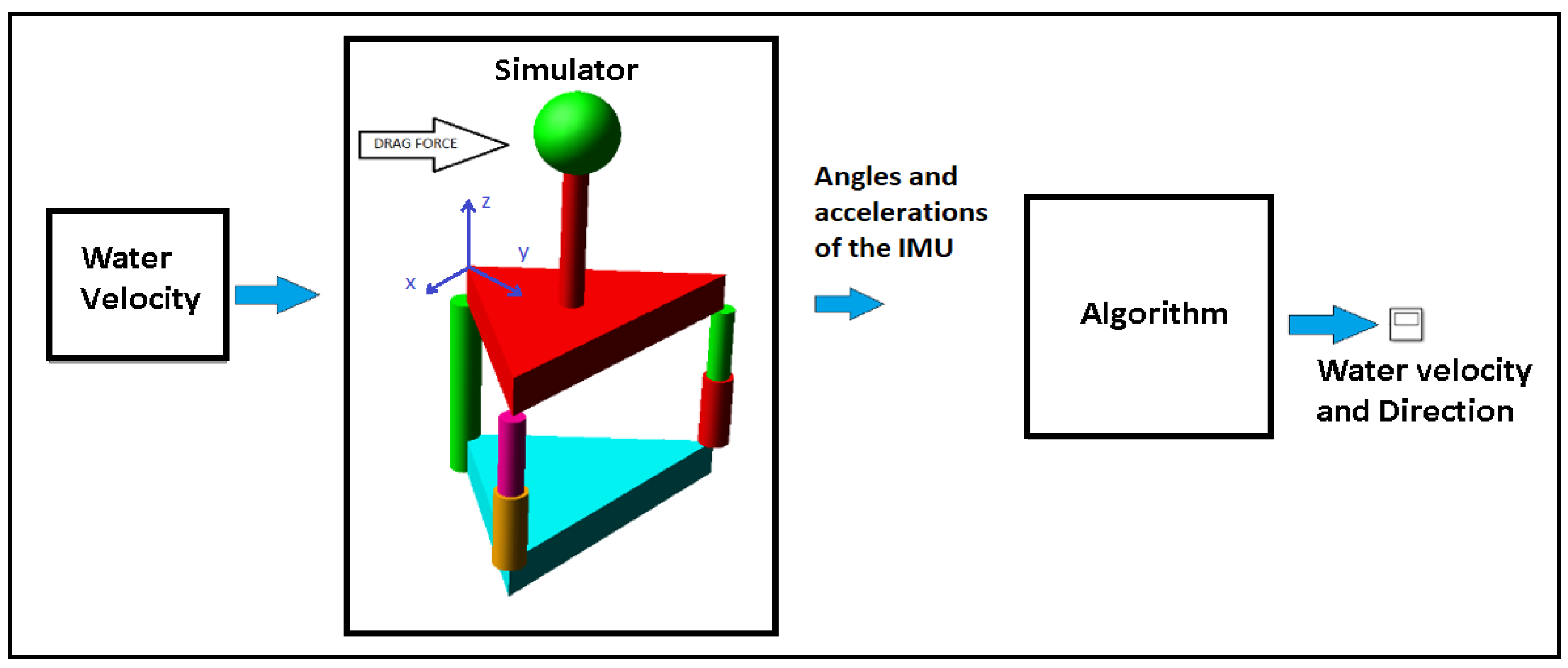
2.4. Practical Implementation and Testing of the Sensor
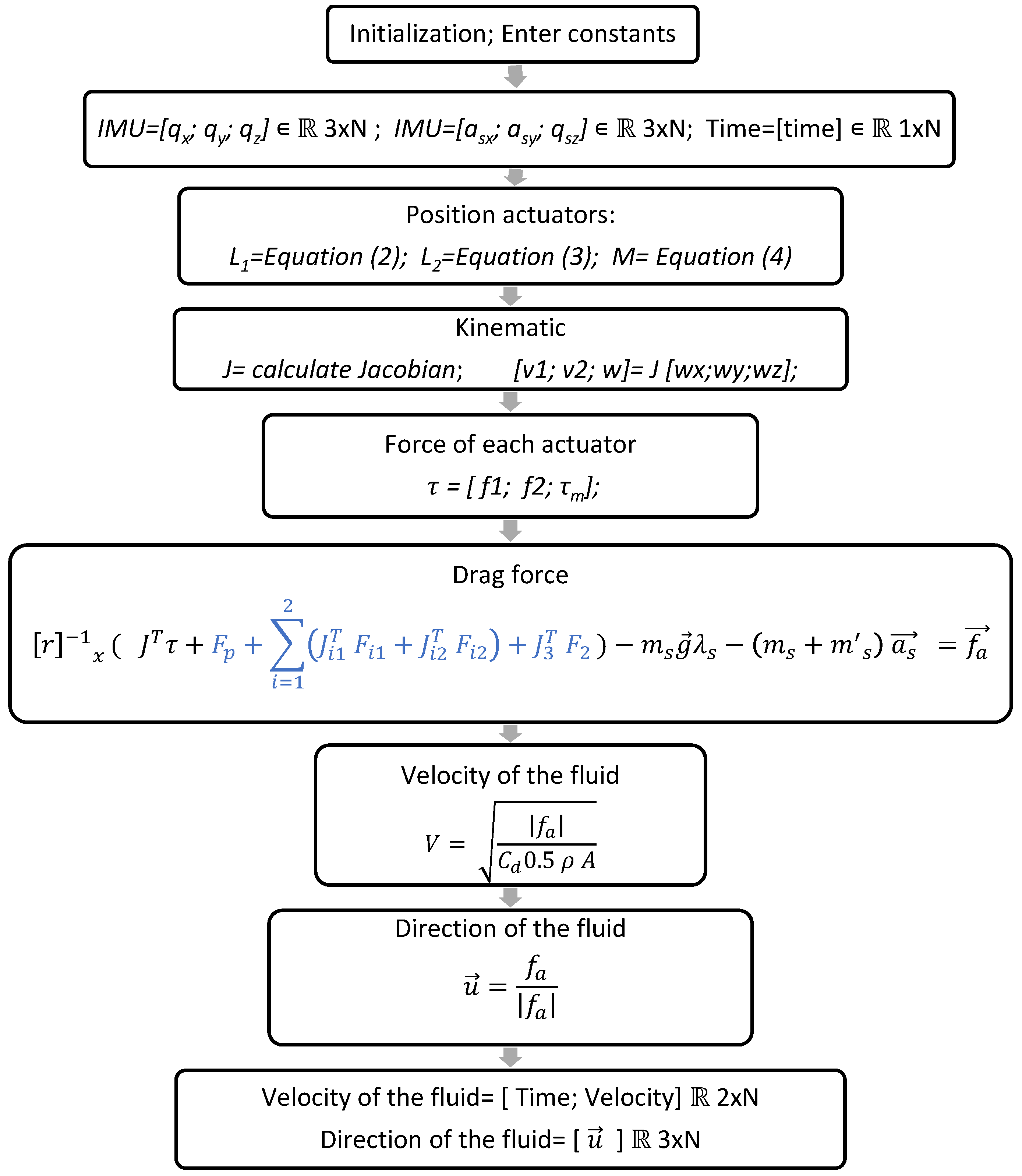
2.4.1. Algorithm for the Sensor
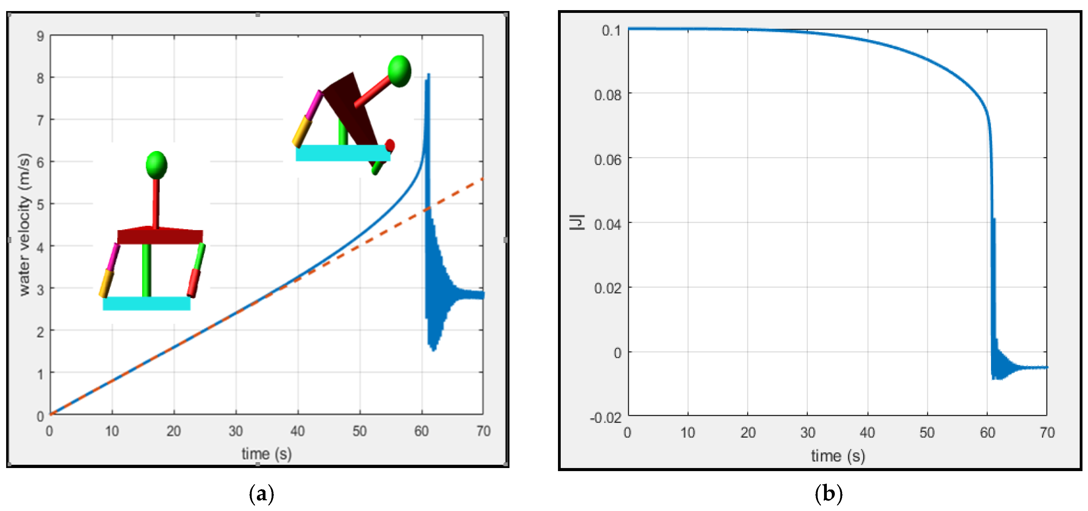
2.4.2. Experiment
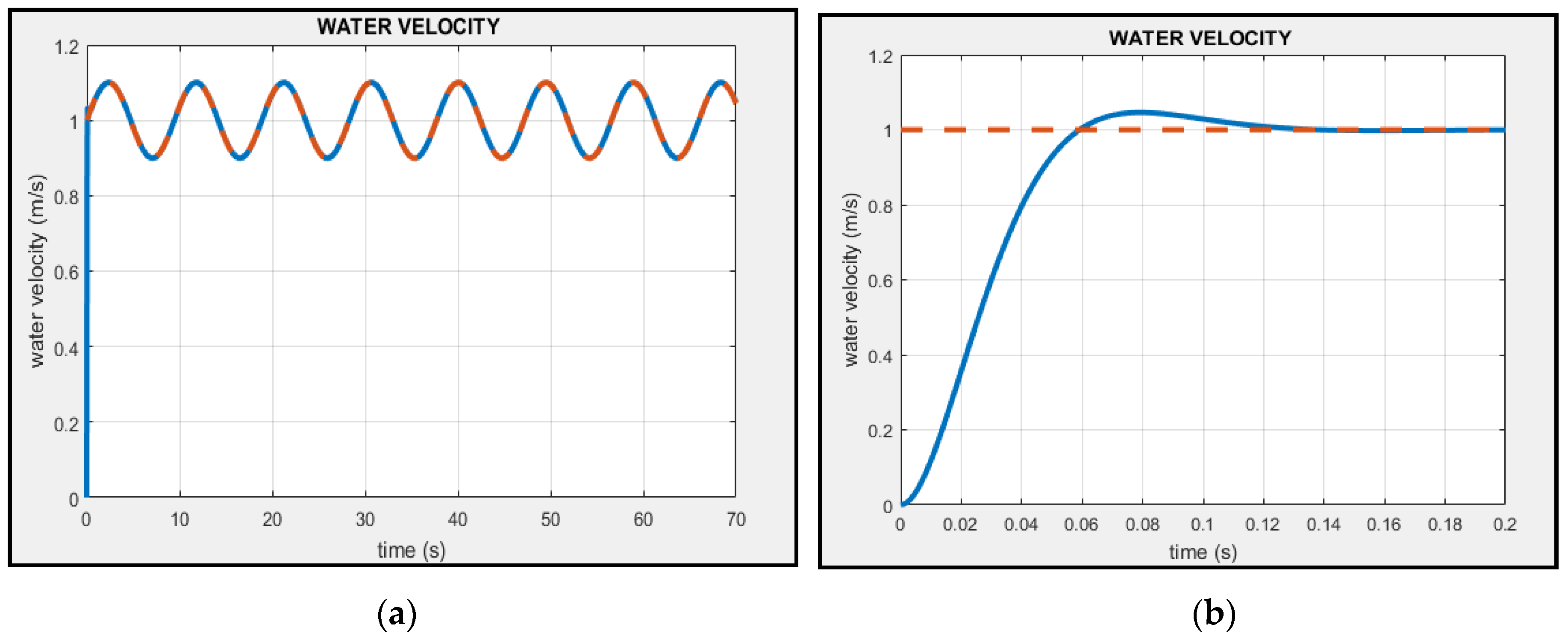
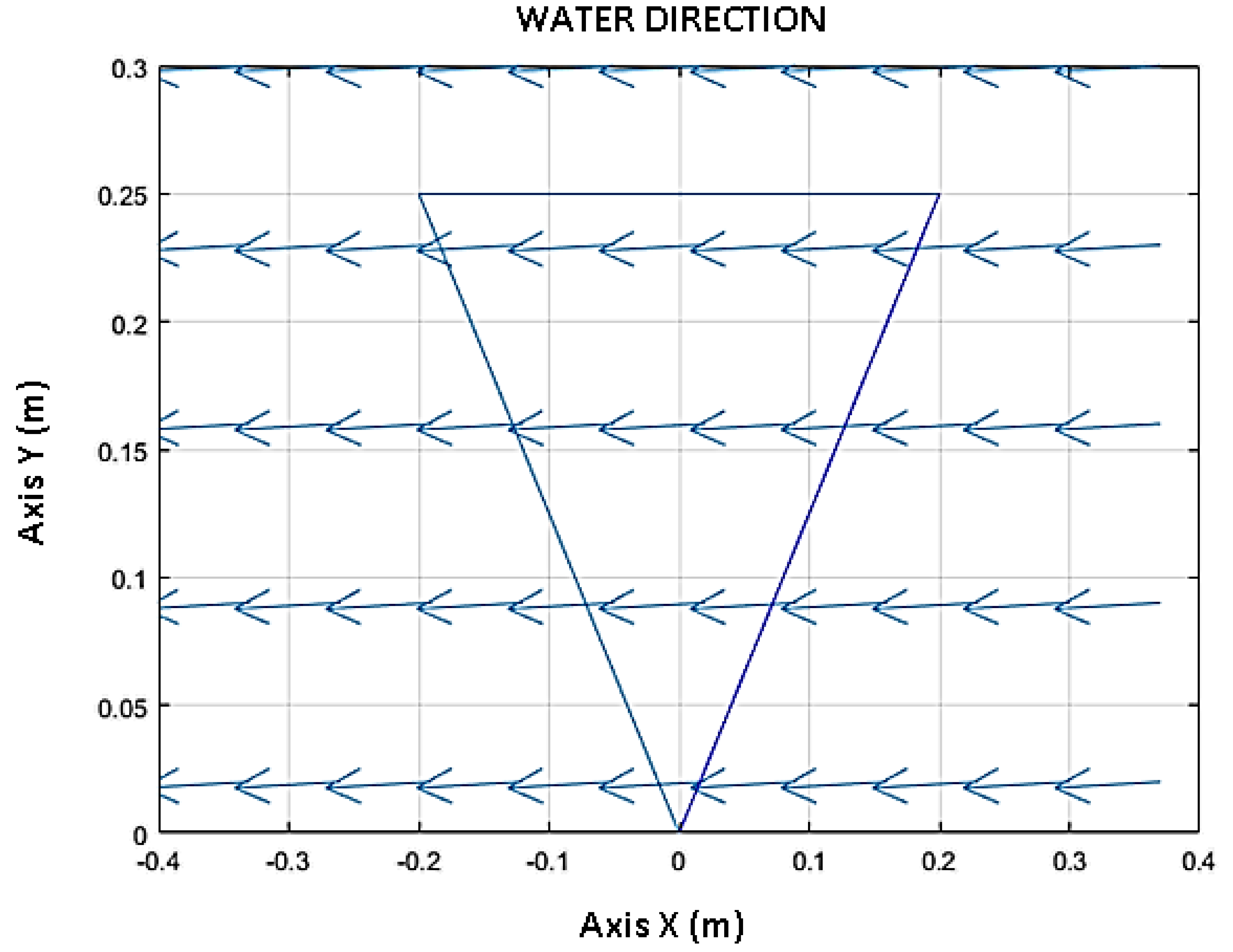
3. Results
4. Discussion
5. Patents
Author Contributions
Funding
Conflicts of Interest
References
- Neauman, G. Ocean Currents; Elsevier: New York, NY, USA, 1968. [Google Scholar]
- Merlet, J.P. Parallel Robots, 2nd ed.; Springer: Dordrecht, The Nertherlands, 2006. [Google Scholar]
- Gough, V.E.; Whitehall, S.G. Universal Tyre Testing Machine; International Technical Congress FISITA; Institution of Mechanical Engineers: London, UK, 1961. [Google Scholar]
- Stewart, D. Platform with six degrees of freedom. Proc. Inst. Mech. Eng. 1965, 180, 371–386. [Google Scholar] [CrossRef]
- Clavel, R. A fast robot with parallel geometry. In Proceedings of the 18th International Symposium on Industrial Robots, Lausanne, France, 26–28 April 1988. [Google Scholar]
- Gosselin, C.M.; Angeles, J. The optimum kinematic design of a spherical three-degree-of-freedom parallel manipulator. J. Mech. Transm. Autom. Des. 1989, 111, 202–207. [Google Scholar] [CrossRef]
- Lande, M.A.; David, R.J. Articulation for manipulator arm. U.S. Patent 4300362, 17 November 1981. [Google Scholar]
- Lu, Y.; Zhang, X.; Sui, C.; Han, J.; Hu, B. Kinematics/statics and workspace analysis of a 3-leg 5-DoF parallel manipulator with a UPU-type composite active constrained leg. Robotica 2013, 31, 183–191. [Google Scholar] [CrossRef]
- Saltaren, R.J.; Sabater, J.M.; Yime, E.; Azorin, J.M.; Aracil, R.; Garcia, N. Performance evaluation of spherical parallel platforms for humanoid robots. Robotica 2006, 25, 257–267. [Google Scholar] [CrossRef]
- Hao, G.; Murphy, M.; Luo, X. Development of a compliant-mechanism-based compact three-axis force sensor for high-precision manufacturing. In Proceedings of the International Design Engineering Technical Conferences and Computers and Information in Engineering Conference, Boston, MA, USA, 2–5 August 2015; American Society of Mechanical Engineers: New York, NY, USA, 2015. [Google Scholar]
- Hao, G.; Kong, X. A normalization-based approach to the mobility analysis of spatial compliant multi-beam modules. Mech. Mach. Theory 2013, 59, 1–9. [Google Scholar] [CrossRef]
- Yang, E. Design and Sensitivity Analysis Simulation of a Novel 3D Force Sensor Based on a Parallel Mechanism. Sensors 2016, 16, 2147. [Google Scholar] [CrossRef] [PubMed]
- Yao, J.T.; Hou, Y.L.; Chen, J.; Lu, L.; Zhao, Y.S. Theoretical analysis and experiment research of a statically indeterminate pre-stressed six-axis force sensor. Sens. Actuators A Phys. 2009, 150, 1–11. [Google Scholar] [CrossRef]
- Lu, Y.; Wang, Y.; Ye, N.; Chen, L. Development of a novel sensor for hybrid hand with three fingers and analysis of its measure performances. Mech. Syst. Signal Process. 2017, 83, 116–129. [Google Scholar] [CrossRef]
- Álvarez, C.; Saltaren, R.; Aracil, R.; García, C. Concepción, Desarrollo y Avances en el Control de Navegación de Robots Submarinos Paralelos: El Robot Remo-I. Rev. Iberoam. Autom. Inf. Ind. 2009, 6, 92–100. [Google Scholar] [CrossRef]
- Rundtop, R.; Frank, K. Experimental evaluation of hydroacoustic instruments for ROV navigation along aquaculture net pens. Aquac. Eng. 2016, 74, 143–156. [Google Scholar] [CrossRef]
- Zhao, B.; Blanke, M.; Skjetne, R. Particle filter ROV navigation using hydroacoustic position and speed log measurements. In Proceedings of the American Control Conference (ACC), Montreal, QC, Canada, 27–29 June 2012. [Google Scholar]
- Liu, P.; Wang, B.; Deng, Z.; Fu, M. INS/DVL/PS Tightly Coupled Underwater Navigation Method with Limited DVL Measurements. IEEE Sens. J. 2018, 18, 2994–3002. [Google Scholar] [CrossRef]
- Fu, K.; Gonzalez, R.; Lee, C. ROBOTICS: Control, Snsing, Visión, and Intelligence, 1st ed.; McGraw-Hill Education: New York, NY, USA, 1989. [Google Scholar]
- Wen, L. Robot Analisis, the Mechanics of Serial and Parallel Manipulators; John Wiley & Sons: New York, NY, USA, 1999. [Google Scholar]
- Davidson, J.; Hunt, K. Robots and Screw Theory; Oxford University Press: Oxford, UK, 2002. [Google Scholar]
- Zhao, J.; Feng, Z.; Chu, F. Advanced Theory of Constraint and Motion Analysis for Robots Mechanisms; Academic Press: Cambridge, MA, USA, 2014. [Google Scholar]
- An, H.S.; Lee, J.H.; Lee, C.; Seo, T.W.; Lee, J.W. Geometrical kinematic solution of serial spatial manipulators using screw theory. Mech. Mach. Theory 2017, 116, 404–418. [Google Scholar] [CrossRef]
- Saltarén, R.; Puglisi, L.J.; Sabater, J.M.; Yime, E. Thomás. In Robótica Aplicada; Dextra Editorial: Madrid, Spain, 2017; pp. 314–315. [Google Scholar]
- Alvarado, J.G.; Agundis, A.R.; Garduño, H.R.; Ramírez, B.A. Kinematics of an asymmetrical three-legged parallel manipulator by means of the screw theory. Mech. Mach. Theory 2010, 45, 1013–1023. [Google Scholar] [CrossRef]
- Alvarado, J.G.; Martínez, M.R.; Alici, G. Kinematics and singularity analyses of a 4-dof parallel manipulator using screw theory. Mech. Mach. Theory 2006, 41, 1048–1061. [Google Scholar] [CrossRef]
- Taghirad, H.D. Parallel Robots: Mechanics and Control; CRC Press: New York, NY, USA, 2013. [Google Scholar]
- Franz, Z. Mechanics of Solids and Fluids; Springer: New York, NY, USA, 2012; pp. 225–256. [Google Scholar]
- Antman, S.S.; Osborn, J.E. The principle of virtual work and integral laws of motion. Arch. Ration. Mech. Anal. 1979, 69, 231–262. [Google Scholar] [CrossRef]
- Khalil, W.; Ibrahim, O. General solution for the dynamic modeling of parallel robots. J. Intell. Robot. Syst. 2007, 49, 19–37. [Google Scholar] [CrossRef]
- Mott, R.L. Mecánica de Fluidos Aplicada; Pearson Educación: Naucalpan de Juárez, Mexico, 1996. [Google Scholar]
- Agrawal, A.; Prasad, B.; Viswanathan, V.; Panda, S.K. Dynamic modeling of variable ballast tank for spherical underwater robot. In Proceedings of the International Conference on Industrial Technology, Cape Town, South Africa, 25–28 February 2013. [Google Scholar]
- Feastherstone, R. Rigid Body Dynamics Algorithms; Springer: Sydney, Autralia, 2008. [Google Scholar]
- Antonelli, G. Underwater Robots; Springer: Berlin/Heidelberg, Germany, 2006. [Google Scholar]
- Sumer, B.M.; Fredsoe, J. Hydrodynamics around Cylindrical Structures; World Scientific Publishing: Singapore, 1997. [Google Scholar]
- Kanatani, K. Understanding Geometric Algebra, Japan; CRC Press: New York, NY, USA, 2015. [Google Scholar]
- Mikhailov, M.D.; Silva Freire, A.P. The drag coefficient of a sphere: An approximation using Shanks transform. Powder Technol. 2013, 237, 432–435. [Google Scholar] [CrossRef]
- Ogata, K. Ingeniería de Control Moderna, 5th ed.; Pearson Educación: Madrid, Spain, 2010. [Google Scholar]
- Thomson, W.T. Theory of Vibration with Applications; CRC Press: New York, NY, USA, 1993. [Google Scholar]

| Geometry (m) | Masses (kg) | Spring Constants |
|---|---|---|
| L1 = 0.250 L2 = 0.250 h = 0.25 h = 0.250 b = 0.20 a = 0.40 Diameter of the sphere = 0.1 m | Triangular platforms = 0.1 L1 = 0.2 L2 = 0.2 h = 0.01 h = 0.01 Sphere = 0.001 | = 320 N/m = 8 (N.s)/m = 18.33 (N.m)/° = 0.458 (N.m.s)/° |
© 2018 by the authors. Licensee MDPI, Basel, Switzerland. This article is an open access article distributed under the terms and conditions of the Creative Commons Attribution (CC BY) license (http://creativecommons.org/licenses/by/4.0/).
Share and Cite
Saltarén, R.; Portilla, G.; Barroso, A.R.; Cely, J. A Sensor Based on a Spherical Parallel Mechanism for the Measurement of Fluid Velocity: Physical Modelling and Computational Analysis. Sensors 2018, 18, 2867. https://doi.org/10.3390/s18092867
Saltarén R, Portilla G, Barroso AR, Cely J. A Sensor Based on a Spherical Parallel Mechanism for the Measurement of Fluid Velocity: Physical Modelling and Computational Analysis. Sensors. 2018; 18(9):2867. https://doi.org/10.3390/s18092867
Chicago/Turabian StyleSaltarén, Roque, Gerardo Portilla, Alejandro R. Barroso, and Juan Cely. 2018. "A Sensor Based on a Spherical Parallel Mechanism for the Measurement of Fluid Velocity: Physical Modelling and Computational Analysis" Sensors 18, no. 9: 2867. https://doi.org/10.3390/s18092867
APA StyleSaltarén, R., Portilla, G., Barroso, A. R., & Cely, J. (2018). A Sensor Based on a Spherical Parallel Mechanism for the Measurement of Fluid Velocity: Physical Modelling and Computational Analysis. Sensors, 18(9), 2867. https://doi.org/10.3390/s18092867