An Improved Velocity Estimation Method for Wideband Multi-Highlight Target Echoes in Active Sonar Systems


Abstract
:1. Introduction
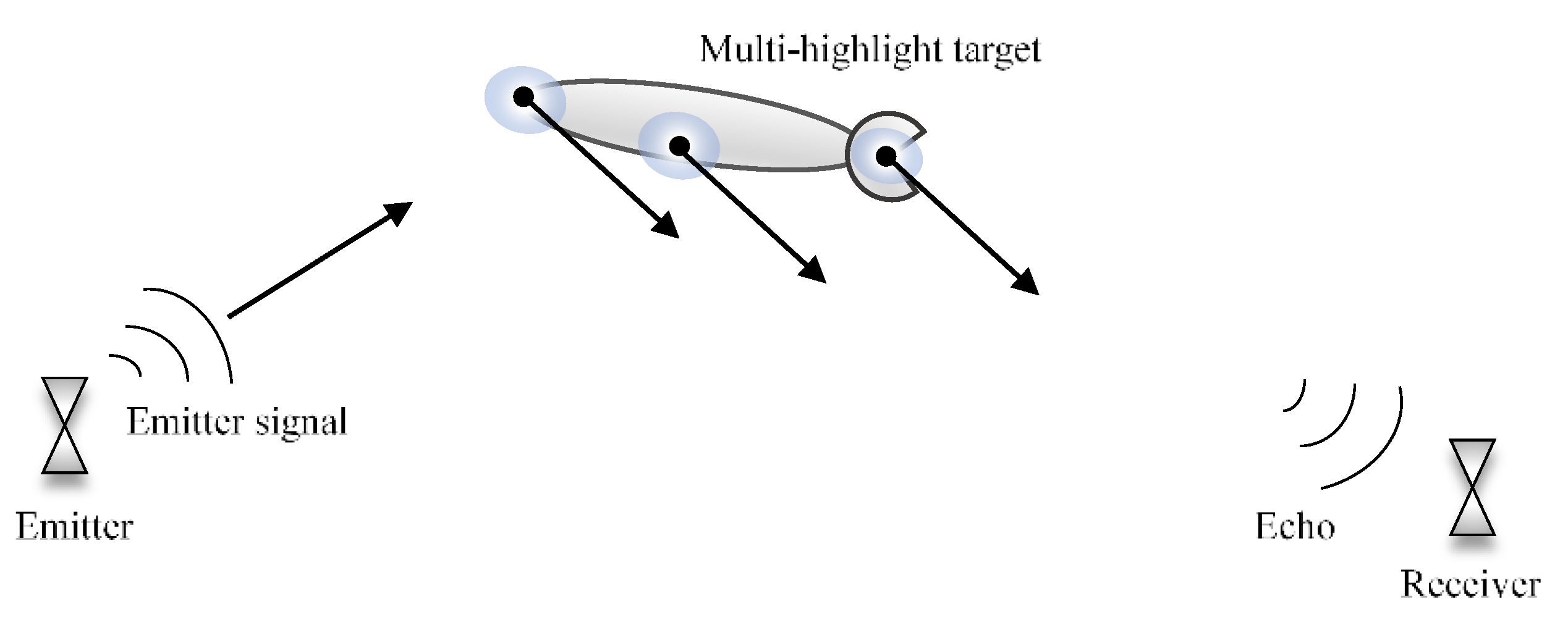
2. An Underwater Echo Model of Multi-Highlight Doppler Targets
3. Wideband Ambiguity Function (WBAF) and Matched Filter (MF) Output
3.1. Basic Theory of MF and WBAF
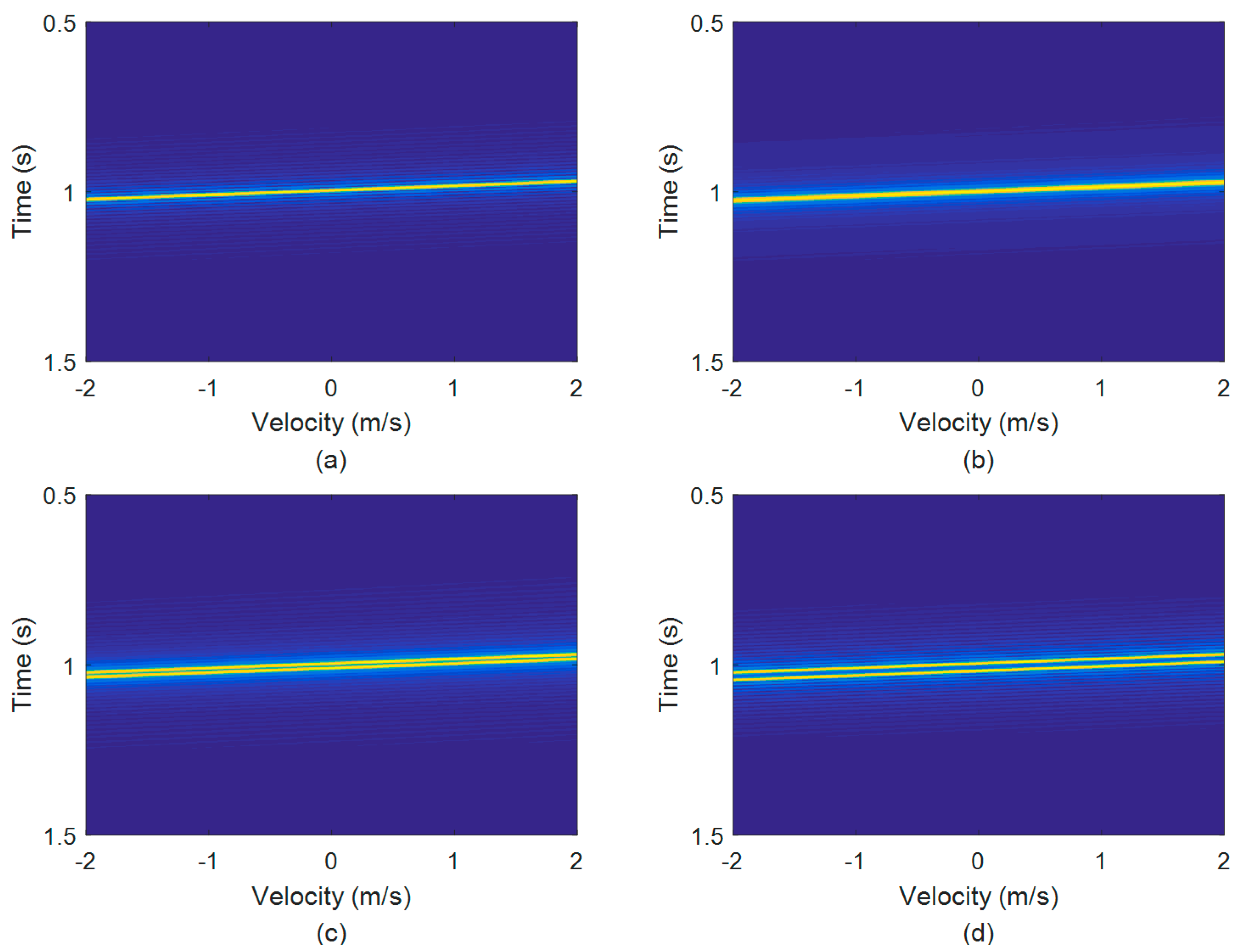
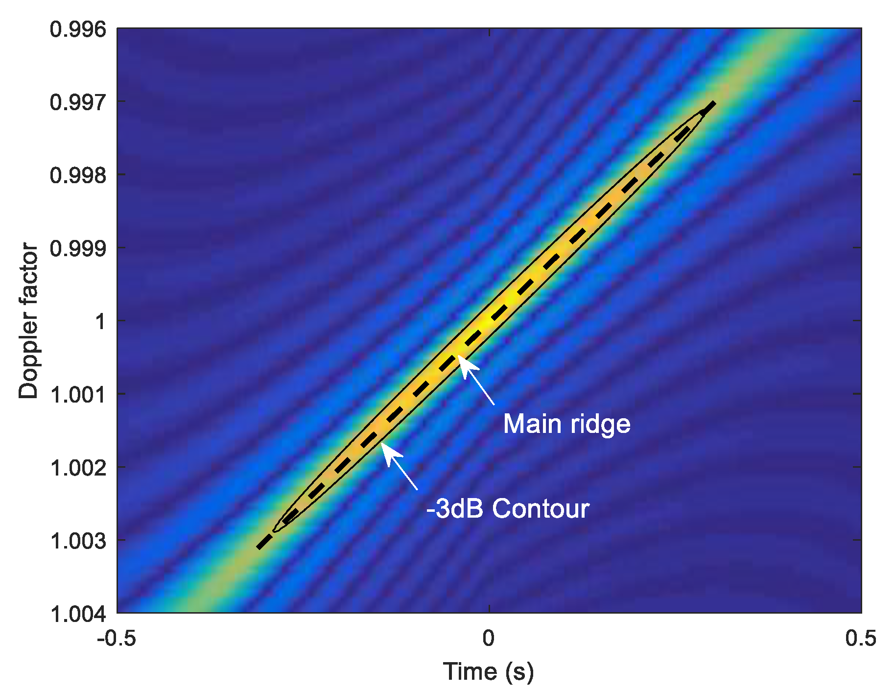
3.2. The WBAF and Doppler Feature of HFM Signal
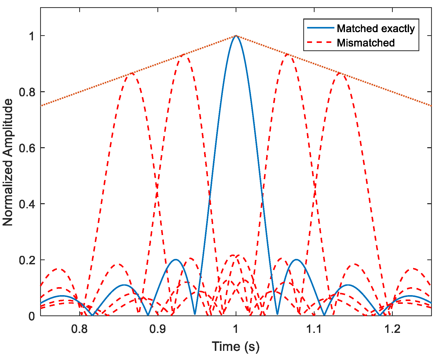
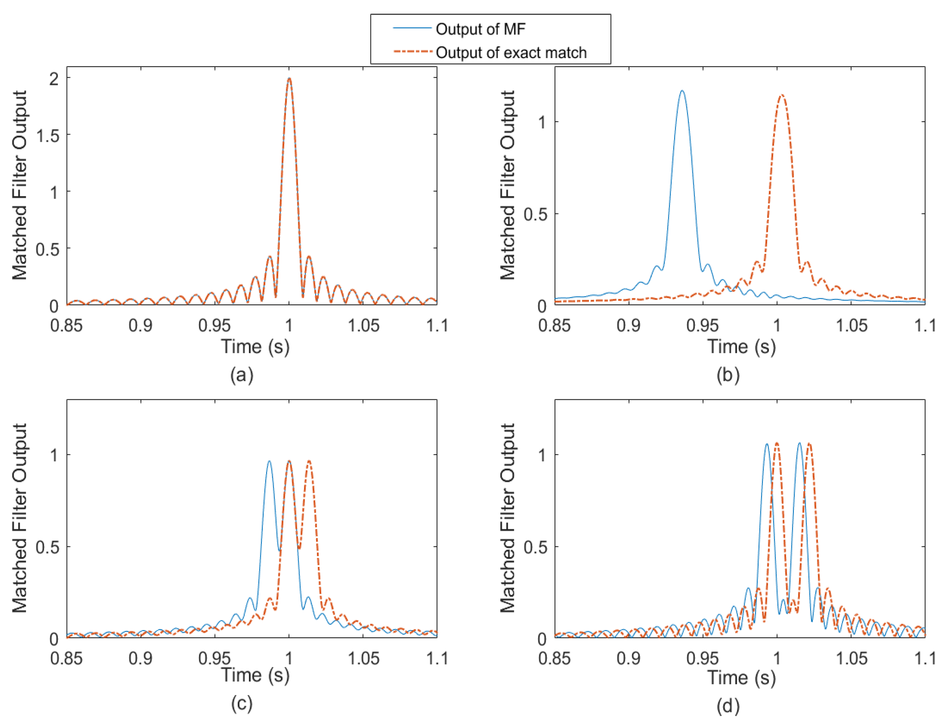
3.3. The MF Output and the WBAF of Wideband Multi-Highlight Echo
4. Velocity Estimation Methods of Multi-Highlight Target with HFM Waveform
4.1. The Matched Fitler (MF) Method
4.2. Focusing on the Dominant Highlight
4.3. The Improved Method
- Step 1.
- Compute the correlation between the echo and the emitter signal to consider the dominant highlight. Then extract the arrival time of the dominant highlight from the MF output.
- Step 2.
- Build the complete dictionary of the copied signals, as introduced in Section 4.1.
- Step 3.
- Compute the time coordinate bias of the dominant highlight, the formula is given as follows:Equation (20) is derived from Equation (13), which is a deduced theoretical conclusion of HFM signal.Cut off the echo by a time window, where the window length is , the starting time of the window is:Set the sampling values outside the window as zero, and then a new echo is constructed:Scan the dictionary and compute the MF outputs times to prepare for the estimation in the next step.
- Step 4.
- Extract the correlation peak values of the MF outputs generated in Step 3 to compose the peak value set . The estimated velocity can be obtained through the comparison among the peak values in , as expressed in Equations (18) and (19).
5. Simulations and Underwater Application
5.1. The Simulations of the MF and Improved Methods
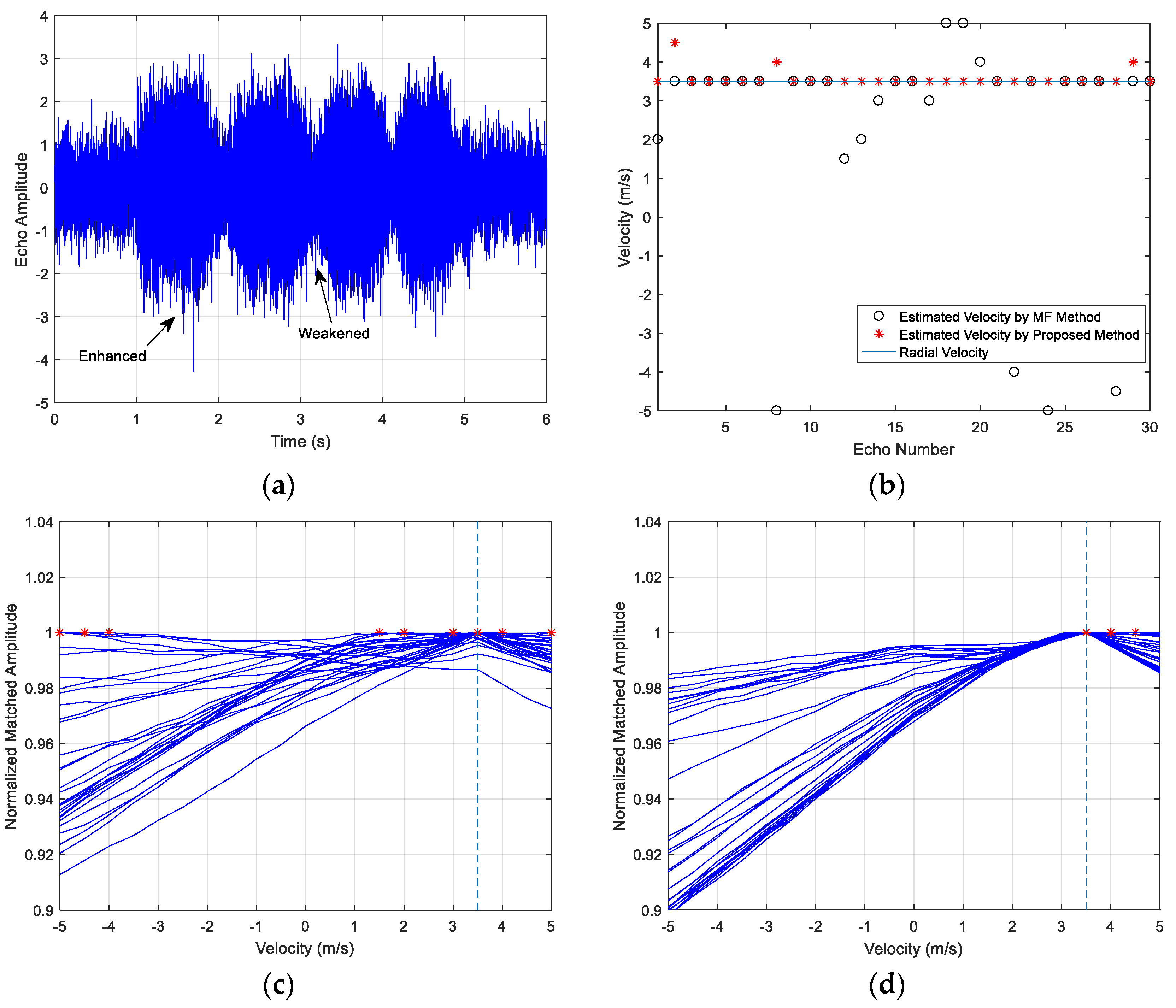
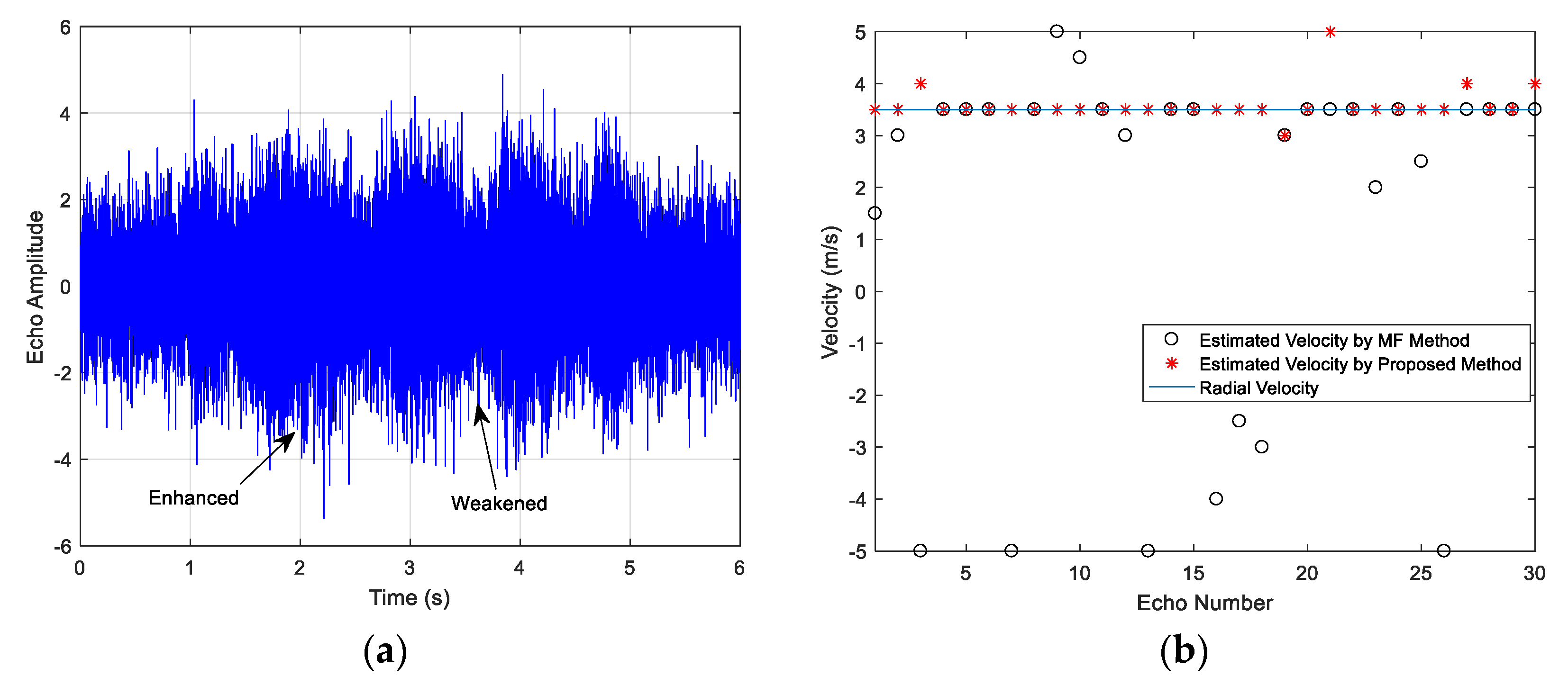
- Case 1: ;
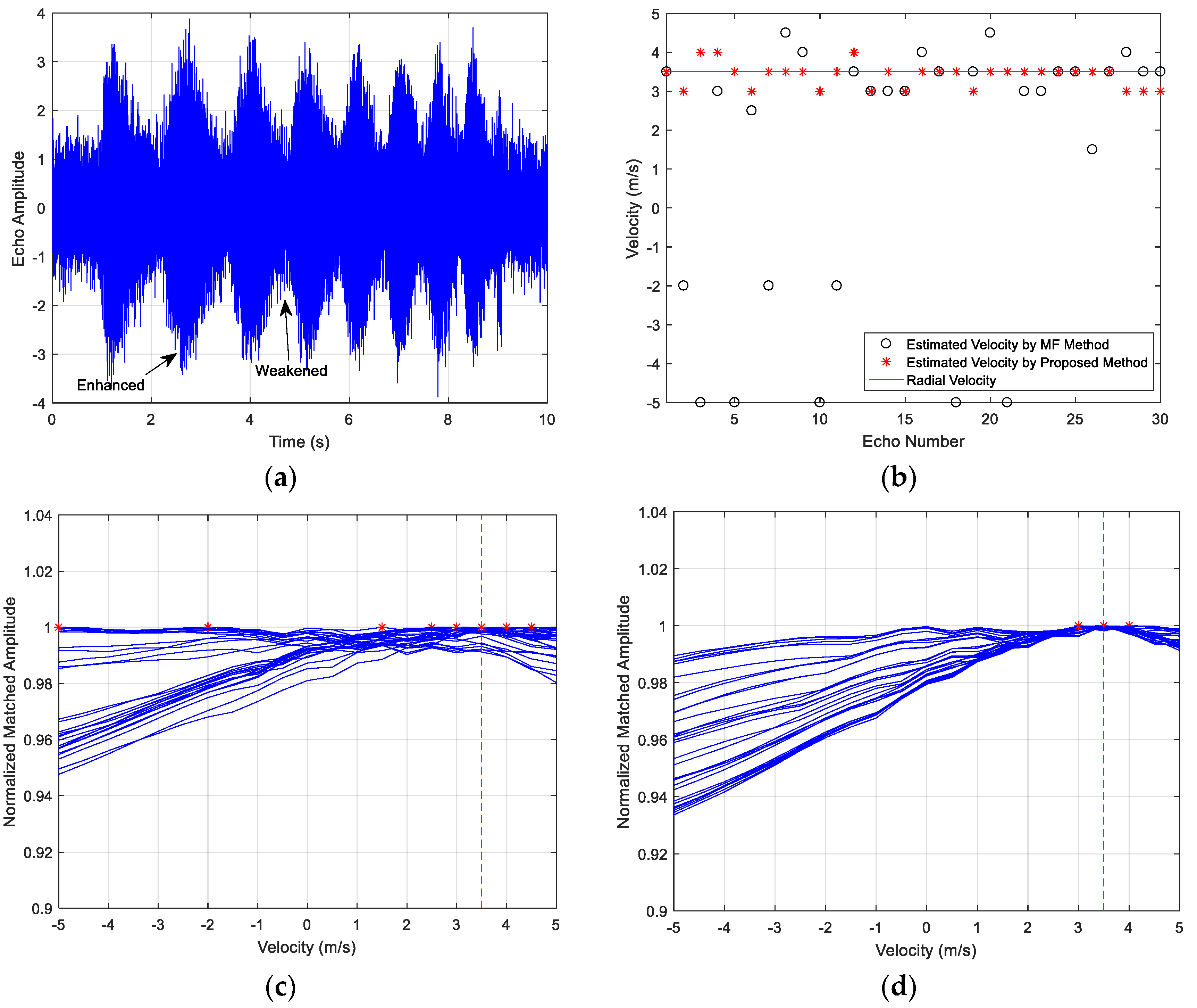
- Case 2: ;
- Case 3: .
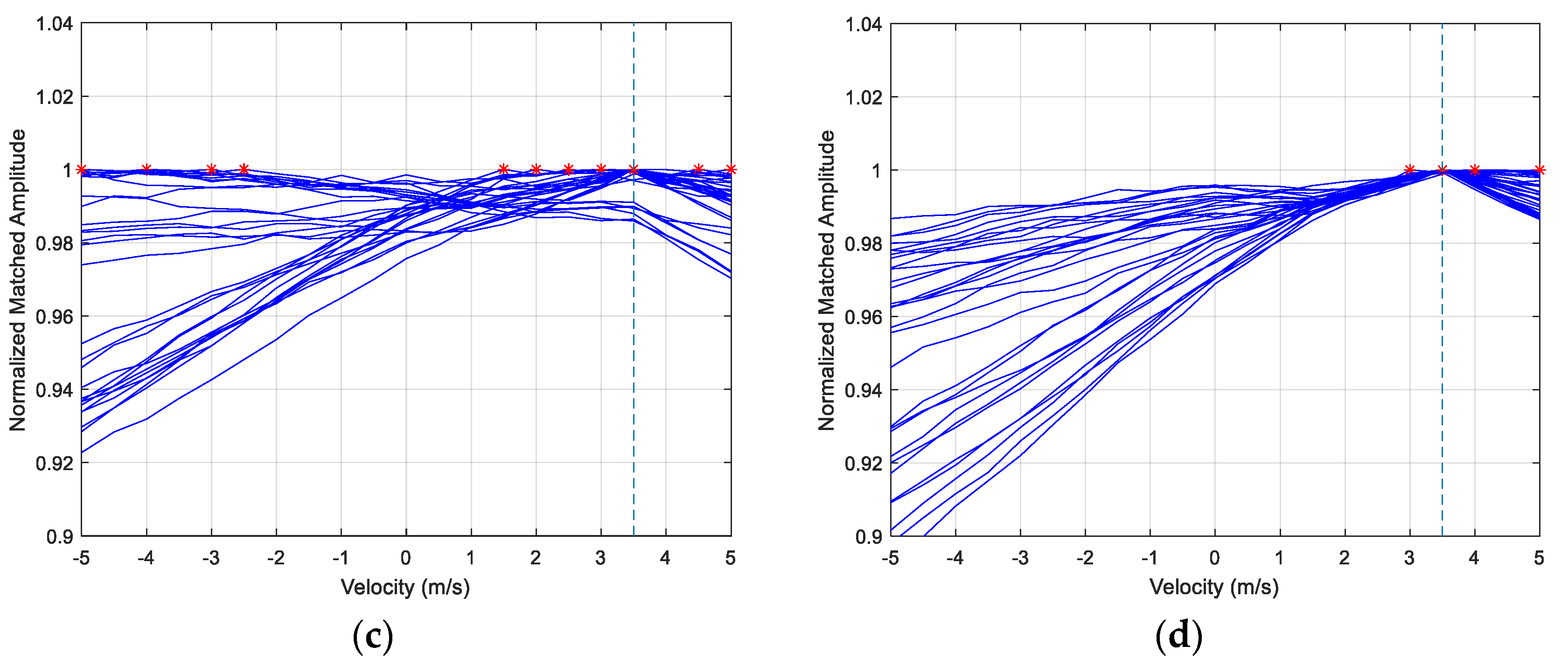
- The estimated velocity values distribute on both sides of the actual radial value. Many estimations of the MF method are outliers, and the results have the biggest estimation errors in the three cases. The accuracy of the proposed method results is improved obviously and it provides a more accurate estimation.
- The estimation accuracy decreases along with the SNR dropping, as shown in the comparison between Case 1 and Case 2, and the target reflection impulses become fuzzy in the received waveforms.
- The estimation accuracy of Case 3 is slightly worse than Case 1, since the power loss ratio of the Case 3 signal’s WBAF is smaller than the Case 1, which can be deduced in Equation (14). The power loss ratio of WBAF is related to of the signal. The ratio of Case 1 is 3.5, and the ratio of Case 3 is 2. The parameters of the Case 3 signal influence its velocity estimation performance, namely smaller power loss ratio results in worse velocity estimation performance under multi-highlight conditions.
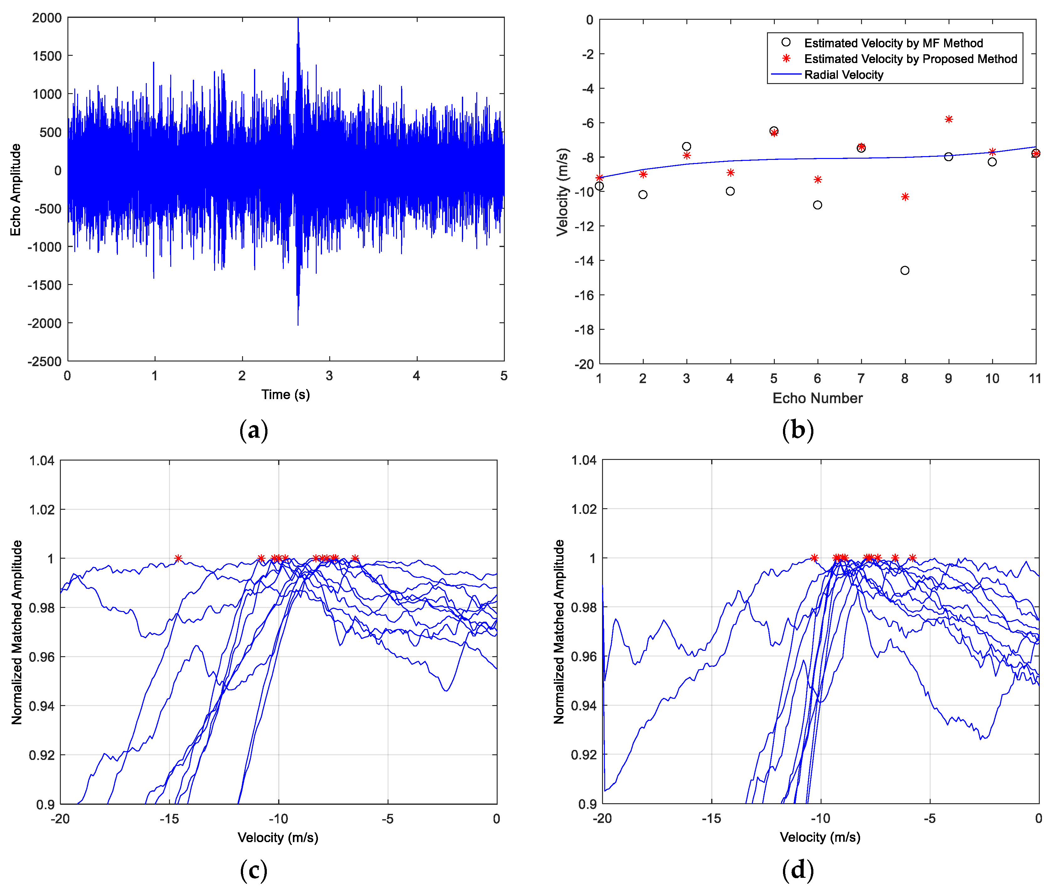
5.2. Application to Underwater Acoustic Data from the Active Sonar 2017 Lake Experiment
6. Conclusions
7. Patents
Author Contributions
Funding
Conflicts of Interest
References
- Chen, X.; Li, Y.A.; Dong, Z.C. Submarine Echo Simulation Method Based on the Highlight Model. In Proceedings of the IEEE International Conference Of IEEE Region 10 (Tencon), Xi’an, China, 22–25 October 2013. [Google Scholar]
- Wu, Y.S.; Li, X.K.; Wang, Y. Extraction and classification of acoustic scattering from underwater target based on Wigner-Ville distribution. Appl. Acoust. 2018, 138, 52–59. [Google Scholar] [CrossRef]
- Yang, M.; Li, X.K.; Yang, Y.; Meng, X.X. Characteristic Analysis of Underwater Acoustic Scattering Echoes in the Wavelet Transform Domain. J. Mar. Sci. Appl. 2017, 16, 93–101. [Google Scholar] [CrossRef]
- Jia, H.J.; Li, X.K.; Meng, X.X. Rigid and elastic acoustic scattering signal separation for underwater target. J. Acoust. Soc. Am. 2017, 142, 653–665. [Google Scholar] [CrossRef] [PubMed]
- Cheng, B.B.; Zhang, H.; Xu, J.; Tang, G.D. Bat Echolocation Signal processing based on Fractional Fourier Transform. In Proceedings of the International Conference on Radar, Adelaide, Australia, 2–5 September 2008. [Google Scholar]
- Kelly, E.J.; Wishner, R.P. Matched-Filter Theory for High-Velocity Accelerating Targets. IEEE Trans. Mil. Electron. 1965, 9, 56–69. [Google Scholar] [CrossRef]
- Adrián-Martínez, S.; Bou-Cabo, M.; Felis, I.; Llorens, C.D.; Martínez-Mora, J.A.; Saldaña, M.; Ardid, M. Acoustic signal detection through the cross-correlation method in experiments with different signal to noise ratio and reverberation conditions. In Proceedings of the International Conference on Ad-Hoc Networks and Wireless, Benidorm, Spain, 22–27 June 2014; pp. 66–79. [Google Scholar]
- Jiang, X.; Zeng, W.J.; Li, X.L. Time delay and Doppler estimation for wideband acoustic signals in multipath environments. J. Acoust. Soc. Am. 2011, 130, 850–857. [Google Scholar] [CrossRef] [PubMed]
- Decultot, D.; Lietard, R.; Maze, G. Classification of a cylindrical target buried in a thin sand-water mixture using acoustic spectra. J. Acoust. Soc. Am. 2010, 127, 1328–1334. [Google Scholar] [CrossRef] [PubMed]
- Sabra, K.G.; Anderson, S.D. Subspace array processing using spatial time-frequency distributions: Applications for denoising structural echoes of elastic targets. J. Acoust. Soc. Am. 2014, 135, 2821–2835. [Google Scholar] [CrossRef] [PubMed]
- Doisy, Y.; Deruaz, L.; Ijsselmuide, S.P.V.; Beerens, S.P.; Been, R. Reverberation Suppression Using Wideband Doppler-Sensitive Pulses. IEEE J. Ocean. Eng. 2008, 33, 419–433. [Google Scholar] [CrossRef]
- Kroszczynski, J.J. Pulse Compression by Means of Linear-Period Modulation. Proc. IEEE 1967, 57, 1260–1266. [Google Scholar] [CrossRef]
- Atkins, P.R.; Collins, T.; Foote, K.G. Transmit-Signal Design and Processing Strategies for Sonar Target Phase Measurement. IEEE J. Sel. Top. Signal Process. 2007, 1, 91–104. [Google Scholar] [CrossRef]
- Doisy, Y.; Deruaz, L.; Beerens, S.P.; Been, R. Target Doppler estimation using wideband frequency modulated signals. IEEE Trans. Signal Process. 2000, 48, 1213–1224. [Google Scholar] [CrossRef]
- Tufts, D.W.; Ge, H.Y.; Umesh, S. Fast Maximum-Likelihood-Estimation of Signal Parameters Using the Shape of the Compressed Likelihood Function. IEEE J. Ocean. Eng. 1993, 18, 388–400. [Google Scholar] [CrossRef]
- Gao, Z.W.; Tao, R.; Wang, Y. Analysis and side peaks identification of Chinese DTTB signal ambiguity functions for passive radar. Sci. China Ser. F 2009, 52, 1409–1417. [Google Scholar] [CrossRef]
- Yan, W.; Huang, J.G.; Wang, X.X.; Hu, F. Simulation and Application of underwater target echo based on highlight model. Comput. Simul. 2005, 10, 23–25. [Google Scholar]
- Ross, R.A. Scattering by a Finite Cylinder. Proc. Inst. Electr. Eng. 1967, 114, 864–868. [Google Scholar] [CrossRef]
- Chen, Y.F.; Li, G.J.; Wang, Z.S.; Zhang, M.W.; Jia, B. Statistical feature of underwater target echo highlight. Acta Phys. Sin. 2013, 62, 084302. [Google Scholar]
- Guo, Q.; Nan, P.L.; Zhang, X.Y.; Zhao, Y.N.; Wan, J. Recognition of Radar Emitter Signals Based on SVD and AF Main Ridge Slice. J. Commun. Netw. 2015, 17, 491–498. [Google Scholar]
- Song, X.F.; Willett, P.; Zhou, S.L. Range Bias Modeling for Hyperbolic-Frequency-Modulated Waveforms in Target Tracking. IEEE J. Ocean. Eng. 2012, 37, 670–679. [Google Scholar] [CrossRef]
- Yang, C.B.; Liang, H. Time-Scale Analysis of Wideband HFM Signal and Application on Moving Target Detection. In Proceedings of the IEEE 4th Conference on Industrial Electronics and Applications, Xi’an, China, 25–27 May 2009. [Google Scholar]
- Josso, N.F.; Ioana, C.; Mars, J.I.; Gervaise, C. Source motion detection, estimation, and compensation for underwater acoustics inversion by wideband ambiguity lag-Doppler filtering. J. Acoust. Soc. Am. 2010, 128, 3416–3425. [Google Scholar] [CrossRef] [PubMed]
- Josso, N.F.; Zhang, J.J.; Papandreou-Suppappola, A.; Ioana, C.; Mars, J.I.; Gervaise, C.; Stephan, Y. On the Characterization of Time-Scale Underwater Acoustic Signals Using Matching Pursuit Decomposition. In Proceedings of the Oceans Conference, Biloxi, MS, USA, 26–29 October 2009. [Google Scholar]
- Zhao, Y.B.; Yu, H.; Wei, G.; Ji, F.; Chen, F.J. Parameter Estimation of Wideband Underwater Acoustic Multipath Channels based on Fractional Fourier Transform. IEEE Trans. Signal Process. 2016, 64, 5396–5408. [Google Scholar] [CrossRef]


| Frequency Range (Hz) | Pulse Duration (s) | SNR (dB) | Velocity Estimation MSE | |
|---|---|---|---|---|
| MF Method | Method of Focusing and Sliding Matching | |||
| 300~400 | 4 | 5 | 9.2833 | 0.0148 |
| 300~400 | 4 | 0 | 14.492 | 0.1762 |
| 300~500 | 8 | 5 | 15.375 | 0.1809 |
© 2018 by the authors. Licensee MDPI, Basel, Switzerland. This article is an open access article distributed under the terms and conditions of the Creative Commons Attribution (CC BY) license (http://creativecommons.org/licenses/by/4.0/).
Share and Cite
Huang, S.; Fang, S.; Han, N. An Improved Velocity Estimation Method for Wideband Multi-Highlight Target Echoes in Active Sonar Systems. Sensors 2018, 18, 2794. https://doi.org/10.3390/s18092794
Huang S, Fang S, Han N. An Improved Velocity Estimation Method for Wideband Multi-Highlight Target Echoes in Active Sonar Systems. Sensors. 2018; 18(9):2794. https://doi.org/10.3390/s18092794
Chicago/Turabian StyleHuang, Shuxia, Shiliang Fang, and Ning Han. 2018. "An Improved Velocity Estimation Method for Wideband Multi-Highlight Target Echoes in Active Sonar Systems" Sensors 18, no. 9: 2794. https://doi.org/10.3390/s18092794
APA StyleHuang, S., Fang, S., & Han, N. (2018). An Improved Velocity Estimation Method for Wideband Multi-Highlight Target Echoes in Active Sonar Systems. Sensors, 18(9), 2794. https://doi.org/10.3390/s18092794