Ambiguity Resolution for Passive 2-D Source Localization with a Uniform Circular Array


Abstract
1. Introduction
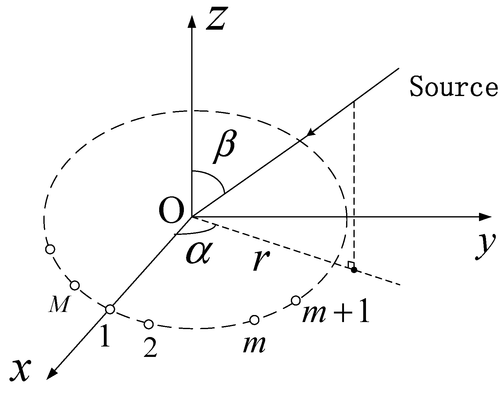
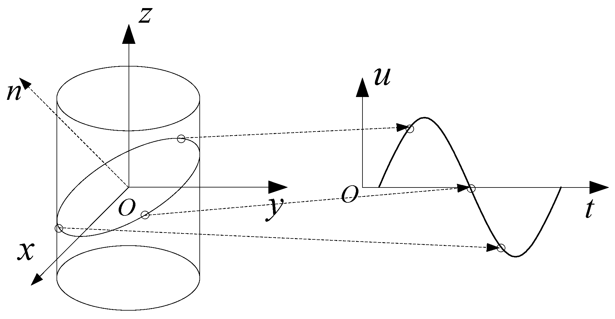
2. Signal Model
3. Ambiguity Resolution of the Source’s Angles
3.1. Phase Difference Estimation
3.2. Ambiguity Resolution Method under the Unambiguous-Relative Phase Observation Model
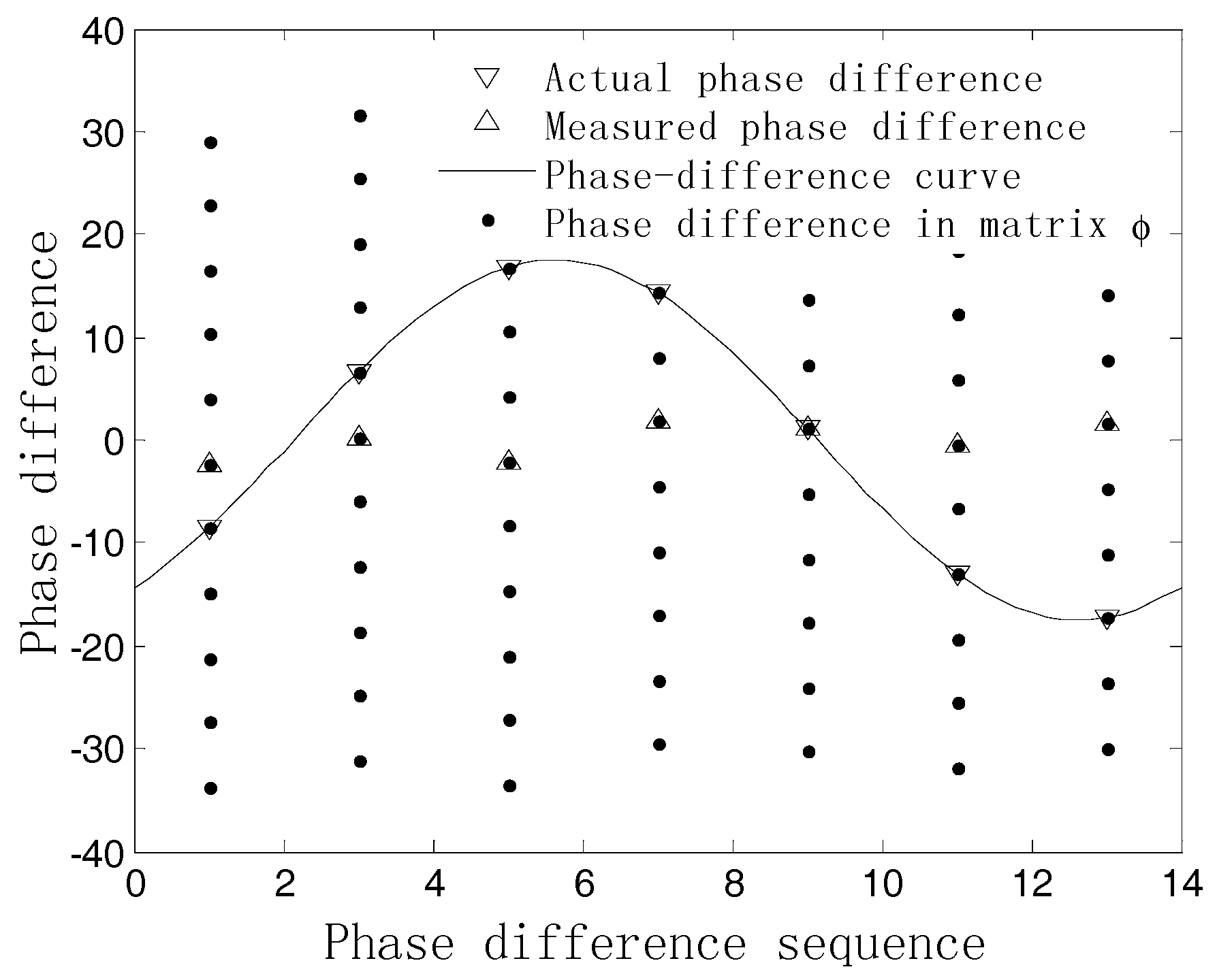
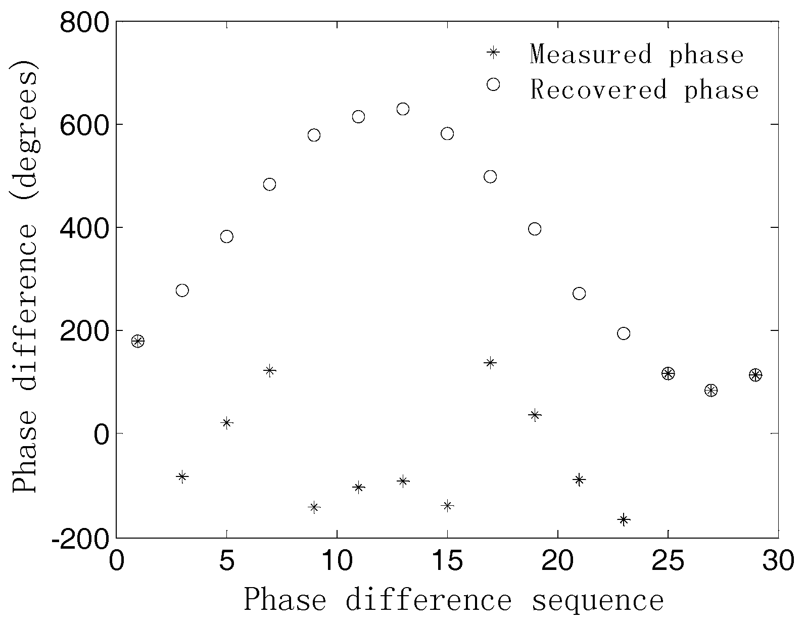
3.3. Ambiguity Resolution Method under the Ambiguous-Relative Phase Observation Model
4. Discussion
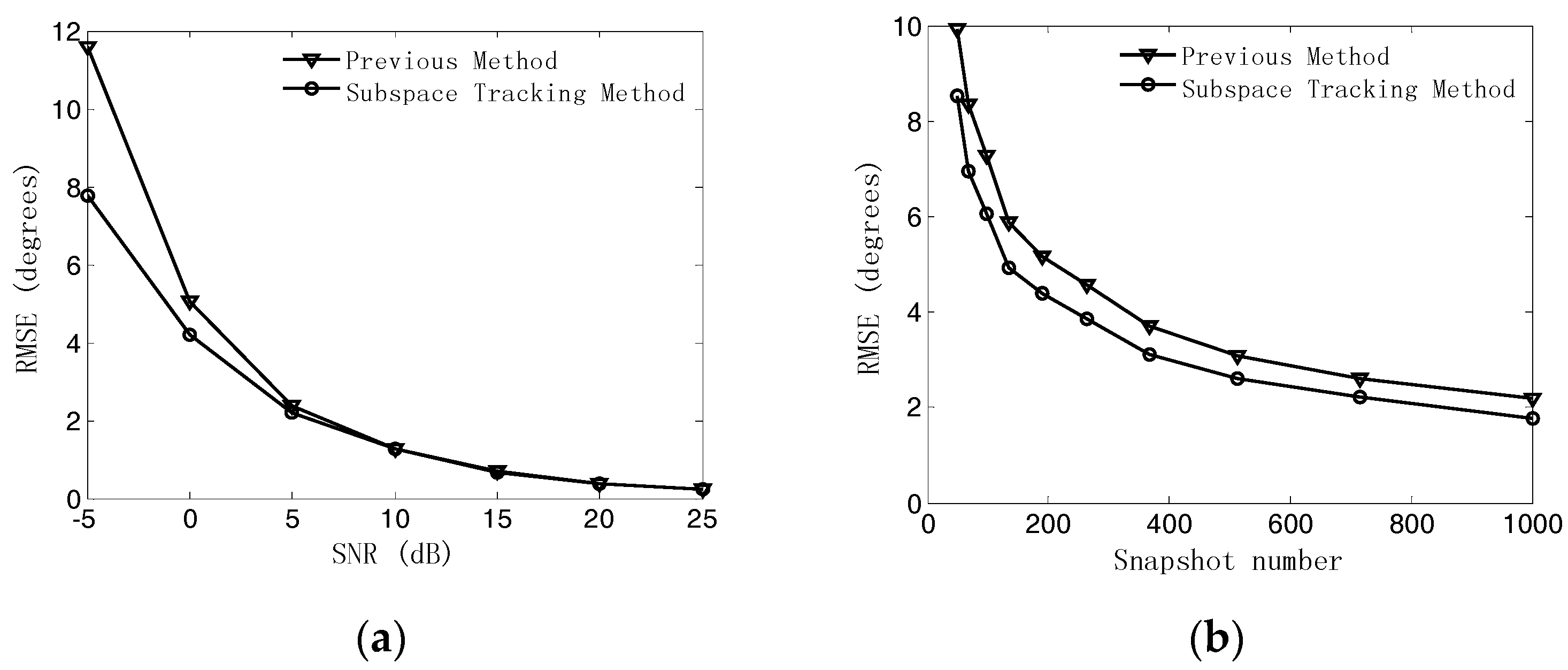
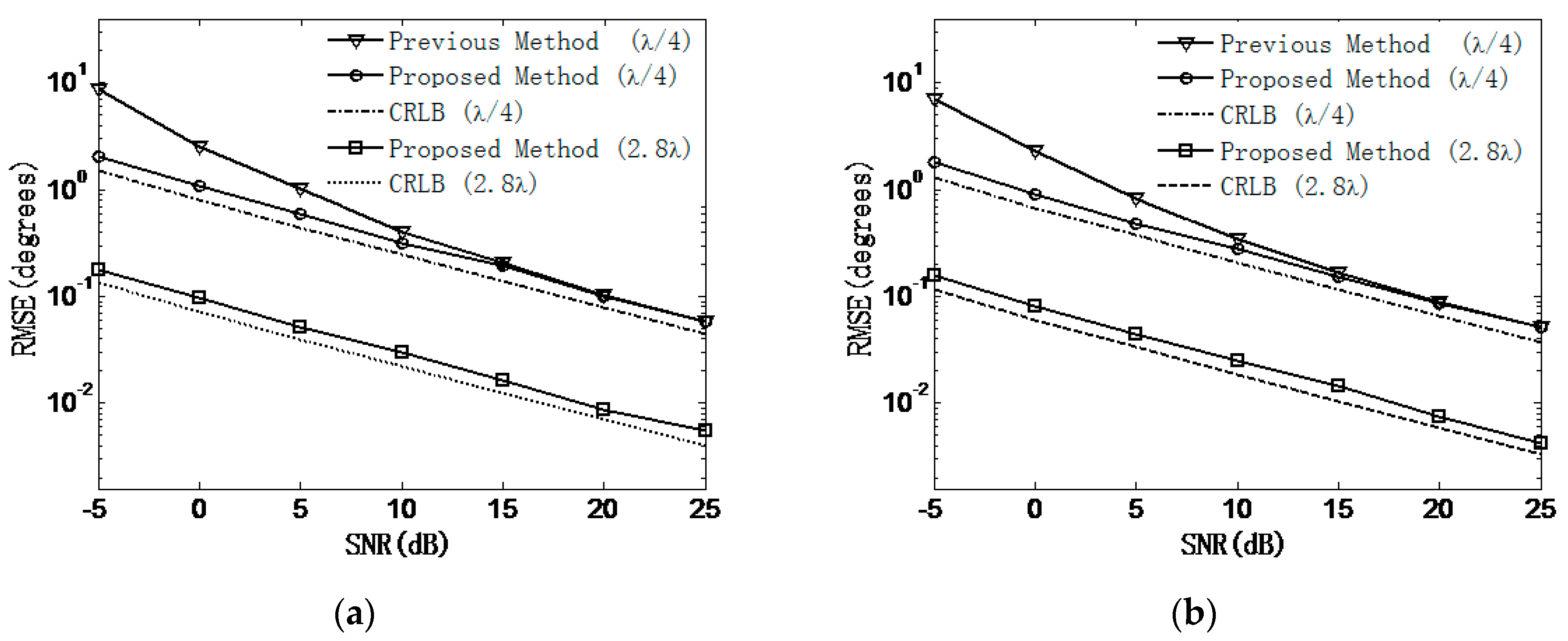
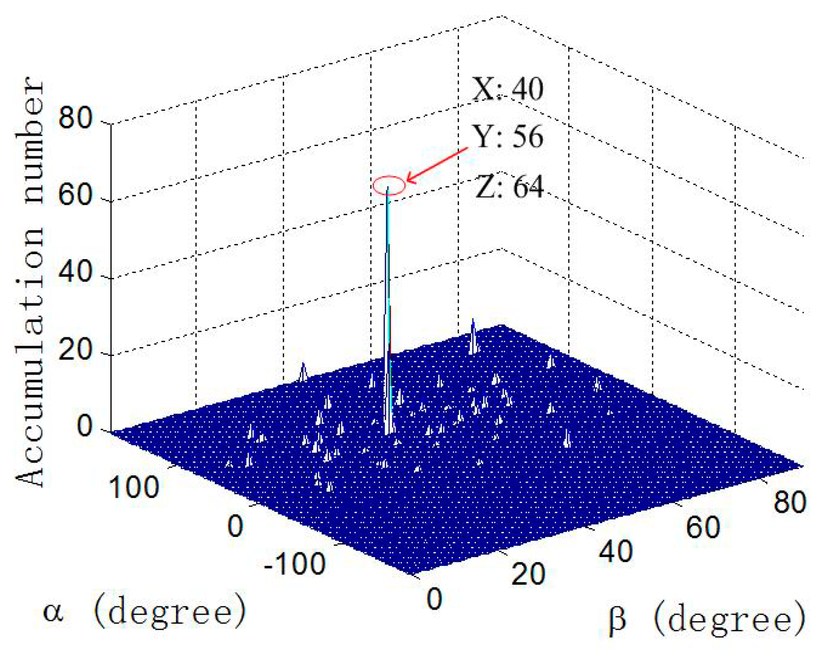
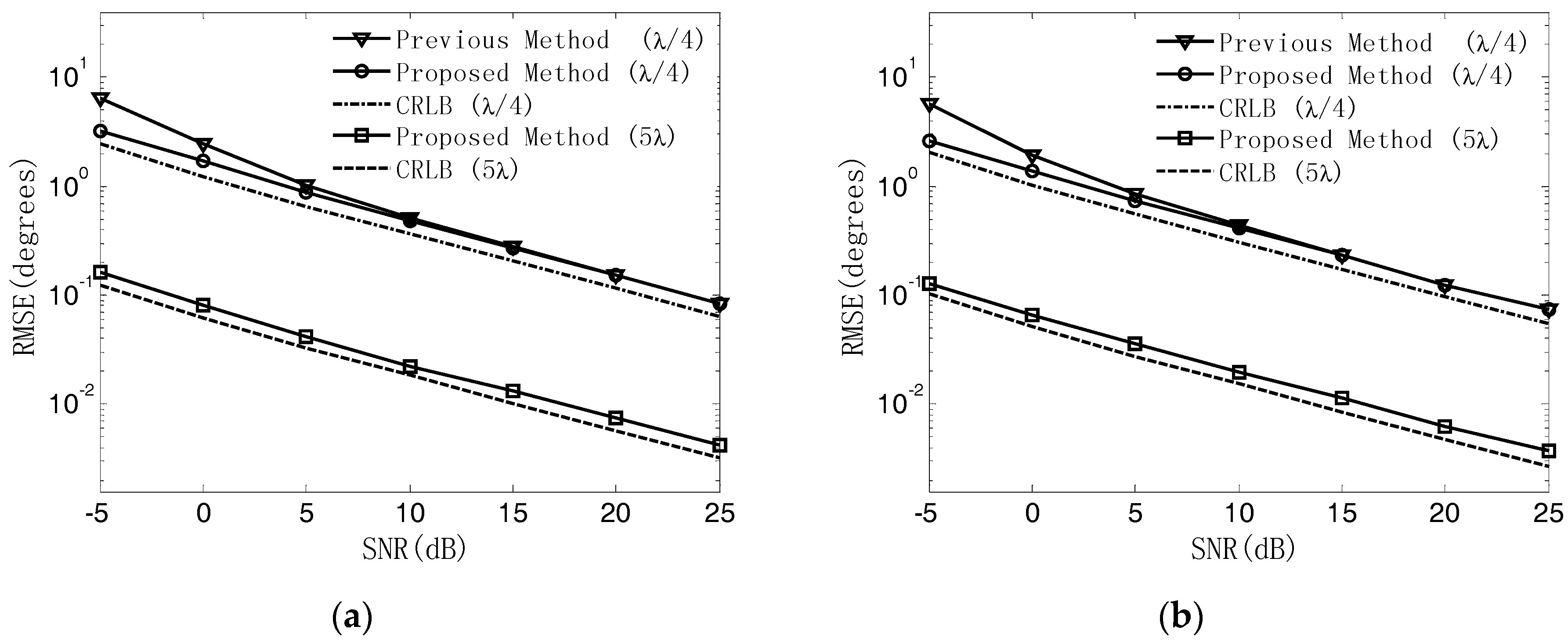
5. Simulation Results
6. Conclusions
Author Contributions
Funding
Acknowledgments
Conflicts of Interest
Appendix A
References
- Krim, H.; Viberg, M. Two decades of array signal processing: The parametric approach. IEEE Signal Process. Mag. 1996, 13, 67–94. [Google Scholar] [CrossRef]
- Wu, N.; Qu, Z.; Si, W.; Jiao, S. DOA and polarization estimation using an electromagnetic vector sensor uniform circular array based on the ESPRIT algorithm. Sensors 2016, 16, 2109. [Google Scholar] [CrossRef] [PubMed]
- Schmidt, R.O. Multiple emitter location and signal parameter estimation. IEEE Trans. Antennas Propag. 1986, 34, 276–280. [Google Scholar] [CrossRef]
- Mathews, C.P.; Zoltowski, M.D. Eigenstructure techniques for 2-D angle estimation with uniform circular arrays. IEEE Trans. Signal Process. 1994, 42, 2395–2407. [Google Scholar] [CrossRef]
- Ye, Z.F.; Xiang, L.; Xu, X. DOA estimation with circular array via spatial averaging algorithm. IEEE Antennas Wirel. Propag. Lett. 2007, 6, 74–76. [Google Scholar] [CrossRef]
- Fuchs, J.-J. On the application of the global matched filter to DOA estimation with uniform circular arrays. IEEE Trans. Signal Process. 2001, 49, 702–709. [Google Scholar] [CrossRef]
- Wu, Y.T.; So, H.C. Simple and accurate two-dimensional angle estimation for a single source with uniform circular array. IEEE Antennas Wirel. Propag. Lett. 2008, 7, 78–80. [Google Scholar] [CrossRef]
- Liao, B.; Wu, Y.T.; Chan, S.C. A generalized algorithm for fast two-dimensional angle estimation of a single source with uniform circular arrays. IEEE Antennas Wirel. Propag. Lett. 2012, 11, 984–986. [Google Scholar] [CrossRef][Green Version]
- Friedlander, B.; Zeira, A. Eigenstructure-based algorithms for direction finding with time-varying arrays. IEEE Trans. Aerosp. Electron. Syst. 1996, 32, 671–689. [Google Scholar] [CrossRef]
- Sheinvald, J.; Wax, M.; Weiss, A.J. Localization of multiple sources with moving arrays. IEEE Trans. Signal. Process. 1998, 42, 2736–2743. [Google Scholar] [CrossRef]
- Liu, M.Z. Direction-of-arrival estimation with time-varying arrays via Bayesian multitask learning. IEEE Trans. Veh. Technol. 2014, 63, 3762–3773. [Google Scholar] [CrossRef]
- Kawase, S. Radio interferometer for geosynchronous satellite direction finding. IEEE Trans. Aerosp. Electron. Syst. 2007, 43, 443–449. [Google Scholar] [CrossRef]
- Zheng, J.; Liu, Z.H.; Qin, B.; Yu, J.B. Algorithm for passive localization with single observer based on ambiguous phase measured by rotating interferometer. In Proceedings of the IEEE International Conference on Electronic Measurement & Instruments (ICEMI), Harbin, China, 16–19 August 2013; pp. 655–659. [Google Scholar] [CrossRef]
- Lin, M.T.; Liu, P.G.; Liu, J.B. Rotary way to resolve ambiguity for planar array. In Proceedings of the IEEE International Conference on Signal Processing Communications and Computing (ICSPCC), Guilin, China, 5–8 August 2014; pp. 170–174. [Google Scholar] [CrossRef]
- Liu, M.Z.; Guo, F.C. Azimuth and elevation estimation with rotating long-baseline interferometers. IEEE Trans. Signal Process. 2015, 63, 2405–2419. [Google Scholar] [CrossRef]
- Chen, X.; Liu, Z.; Wei, X.Z. Ambiguity resolution for phase-based 3-D source localization under fixed uniform circular array. Sensors 2017, 17, 1086. [Google Scholar] [CrossRef] [PubMed]
- Wu, Y.T.; Wang, H.; So, H.C. Fast algorithm for three-dimensional single near-field source localization with uniform circular array. In Proceedings of the IEEE CIE International Conference on Radar, Chengdu, China, 24–27 October 2011; pp. 350–352. [Google Scholar] [CrossRef]
- Jung, T.J.; Lee, K.K. Closed-form algorithm for 3-D single-source localization with uniform circular array. IEEE Antennas Wirel. Propag. Lett. 2014, 13, 1096–1099. [Google Scholar] [CrossRef]
- Xenofon, G.D.; George, V.M. Fast and stable subspace tracking. IEEE Trans. Signal Process. 2008, 56, 1452–1465. [Google Scholar] [CrossRef]
- Chen, H.; Wang, Y.L.; Wu, Z.W. Frequency and 2-D angle estimation based on circular array. In Proceedings of the IEEE Antenna and Propagation Society International Symposium, Boston, MA, USA, 14–17 October 2003; pp. 920–923. [Google Scholar] [CrossRef]
- Xu, L.; Oja, E.; Kultanen, P. A new curve detection method: Randomized Hough Transform (RHT). Pattern Recognit. Lett. 1990, 11, 331–338. [Google Scholar] [CrossRef]
- Liu, J.; Ma, L.; Liu, Z.X.; Wang, X.S.; Wang, G.Y. Detection of zero baseline sinusoidal curve based on Randomized Hough Transform. Comput. Eng. 2010, 36, 1–3. [Google Scholar]
- Gazzah, H.; Abed-Meraim, K. Optimum ambiguity free direction and omnidirectional planar antenna arrays for DOA estimation. IEEE Trans. Signal Process. 2009, 57, 3942–3953. [Google Scholar] [CrossRef]


© 2018 by the authors. Licensee MDPI, Basel, Switzerland. This article is an open access article distributed under the terms and conditions of the Creative Commons Attribution (CC BY) license (http://creativecommons.org/licenses/by/4.0/).
Share and Cite
Xin, J.; Liao, G.; Yang, Z.; Shen, H. Ambiguity Resolution for Passive 2-D Source Localization with a Uniform Circular Array. Sensors 2018, 18, 2650. https://doi.org/10.3390/s18082650
Xin J, Liao G, Yang Z, Shen H. Ambiguity Resolution for Passive 2-D Source Localization with a Uniform Circular Array. Sensors. 2018; 18(8):2650. https://doi.org/10.3390/s18082650
Chicago/Turabian StyleXin, Jinlong, Guisheng Liao, Zhiwei Yang, and Haoming Shen. 2018. "Ambiguity Resolution for Passive 2-D Source Localization with a Uniform Circular Array" Sensors 18, no. 8: 2650. https://doi.org/10.3390/s18082650
APA StyleXin, J., Liao, G., Yang, Z., & Shen, H. (2018). Ambiguity Resolution for Passive 2-D Source Localization with a Uniform Circular Array. Sensors, 18(8), 2650. https://doi.org/10.3390/s18082650