A Novel Semi-Supervised Feature Extraction Method and Its Application in Automotive Assembly Fault Diagnosis Based on Vision Sensor Data


Abstract
:1. Introduction
- (1)
- A novel semi-supervised feature extraction method called, SS-CKFDA, was proposed. In order to confirm the method’s effectiveness, a simulation experiment based on TEP data was performed, and the results were compared with three other FDA-based methods.
- (2)
- SS-CKFDA was introduced to mine fault information obtained from the historical data of the hybrid visual inspection system. Based on this, a novel fault diagnosis flow was put forward for automotive body assembly.
- (3)
- A real experimental system for the automotive body assembly process was realized, and the results show that the proposed method can greatly enhance diagnosis accuracy, especially when less labeled data are obtained.
- (4)
- Two representative classifiers, k-nearest neighbor classifier (KNN) and minimum distance classifier (MD), were also discussed in the present study.
2. Methodology
2.1. Principle of the Complete Kernel Fisher Discriminant Analysis (CKFDA)
2.2. Semi-Supervised Complete Kernel Fisher Discriminant Analysis
2.2.1. Semi-Supervised Learning
2.2.2. The SS-CKFDA Algorithm
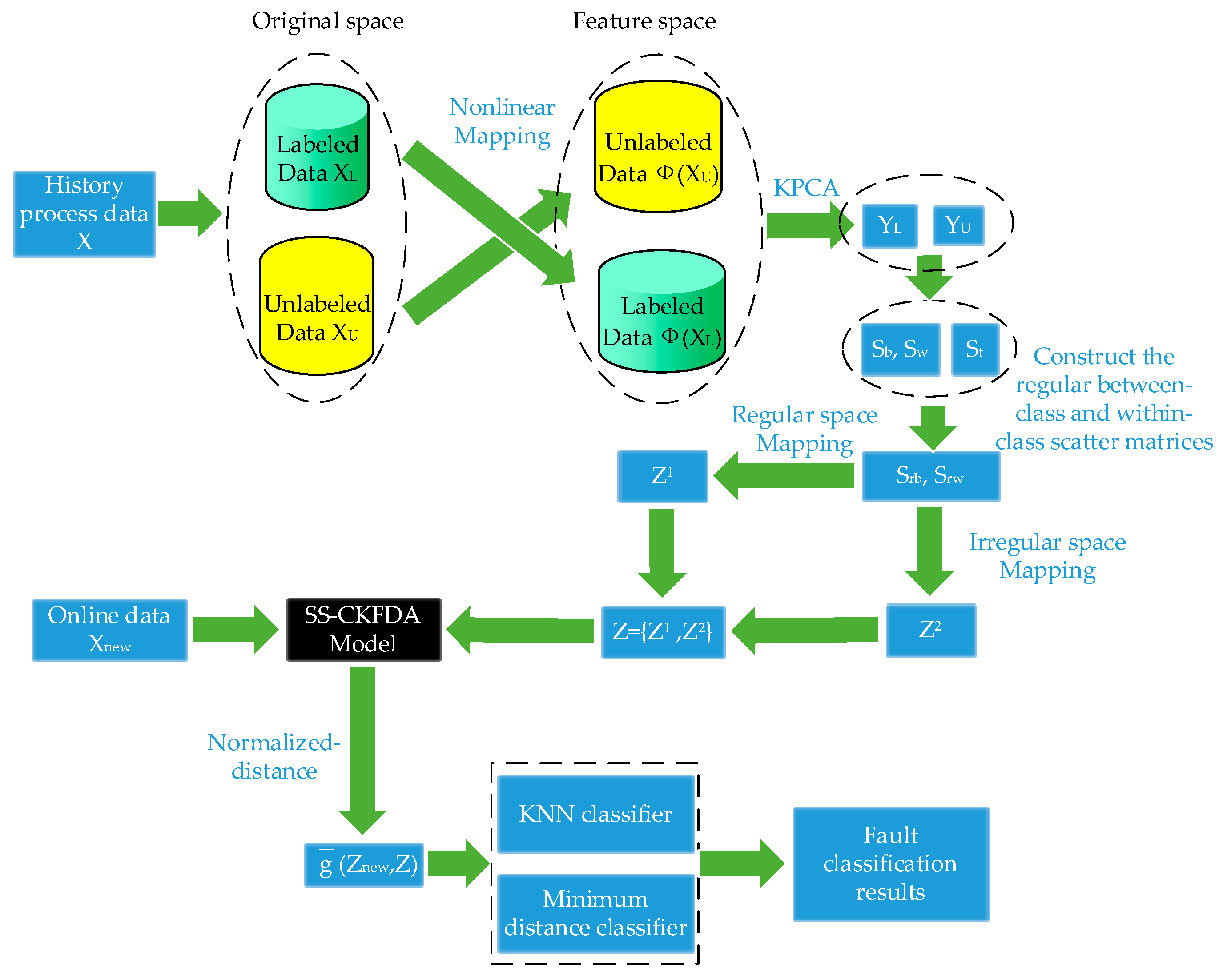
| Algorithm 1. (SS-CKFDA Algorithm): | |
| Step 1: | KPCA is performed for both labeled and unlabeled samples. Data in input space is transformed to data in feature space . |
| Step 2: | SELF is performed in . First, between-class scatter matrices and within-class scatter matrices are constructed with data by Equations (5) and (6). Then, the regular between-class scatter matrices and regular within-class scatter matrices are constructed with data , and by Equations (12) and (13). |
| Step 3: | The ’s orthonormal eigenvectors are calculated, assuming that the first q (q = rank()) corresponds to the positive eigenvalues. |
| Step 4: | The regular discriminant feature is extract in regular space by Equation (9) and irregular discriminant feature is extracted in irregular space by Equation (10). |
| Step 5: | The regular and irregular discriminant features are fused using Equation (11) for classification. |
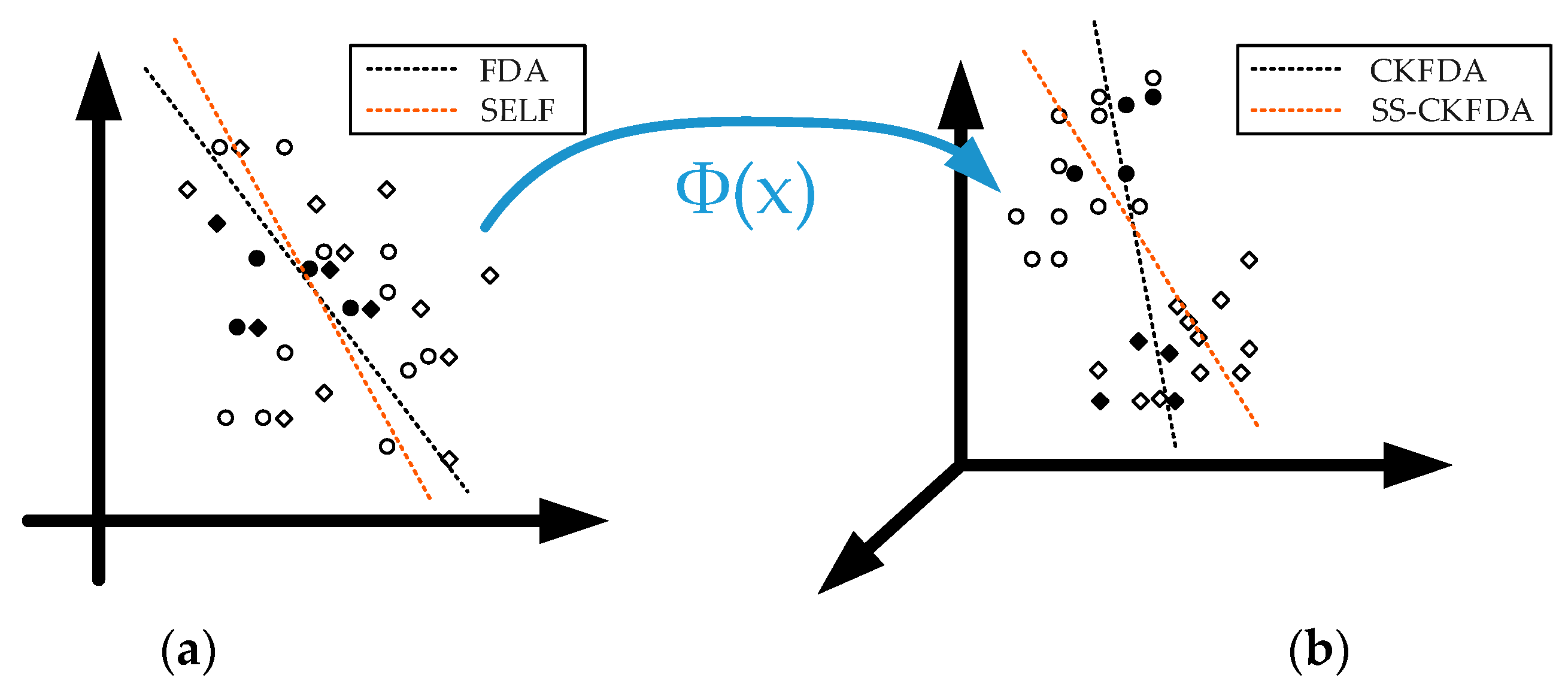
2.2.3. Comparison of SS-CKFDA with Other FDA Algorithms
2.3. SS-CKFDA for Fault Diagnosis
3. Experiment Description
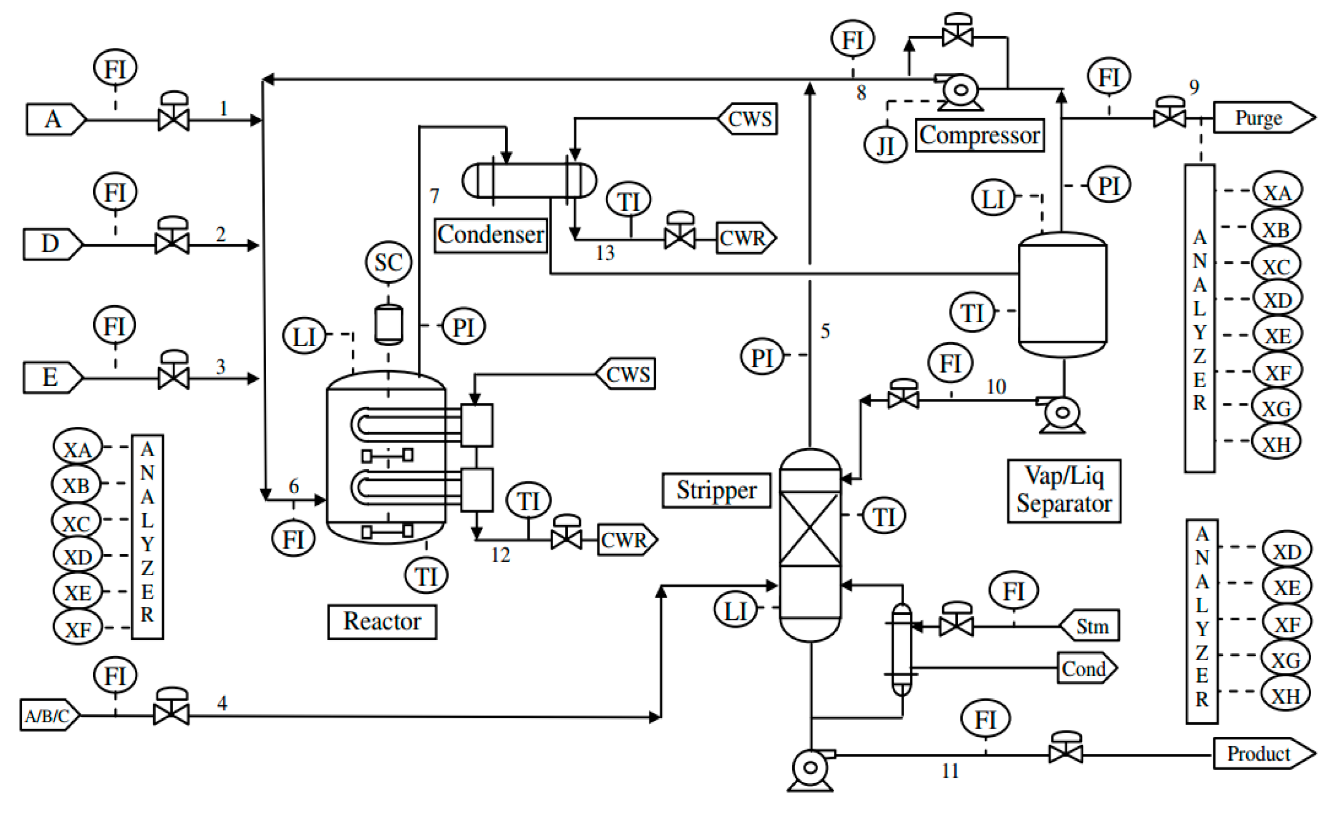
3.1. Experiment I: Tennessee Eastman Process
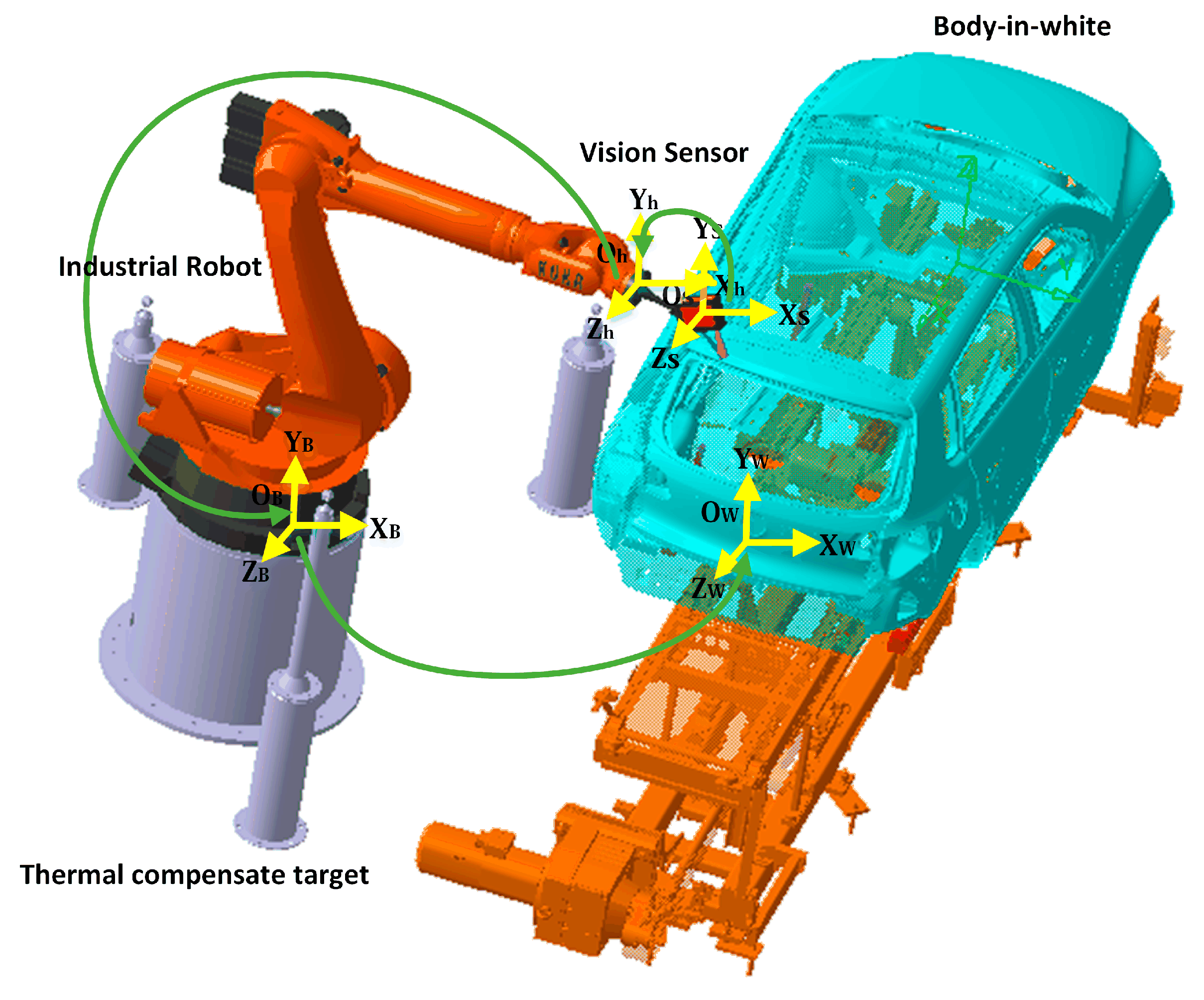
3.2. Experiment II: Automotive Assembly Process
4. Results and Discussion
4.1. Parameter Selection Strategy
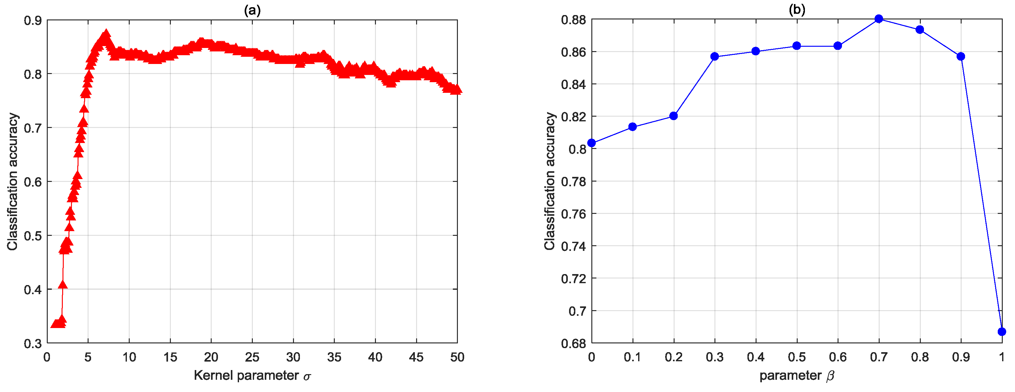
4.1.1. The Effect of Kernel Parameter and Tuning Parameter
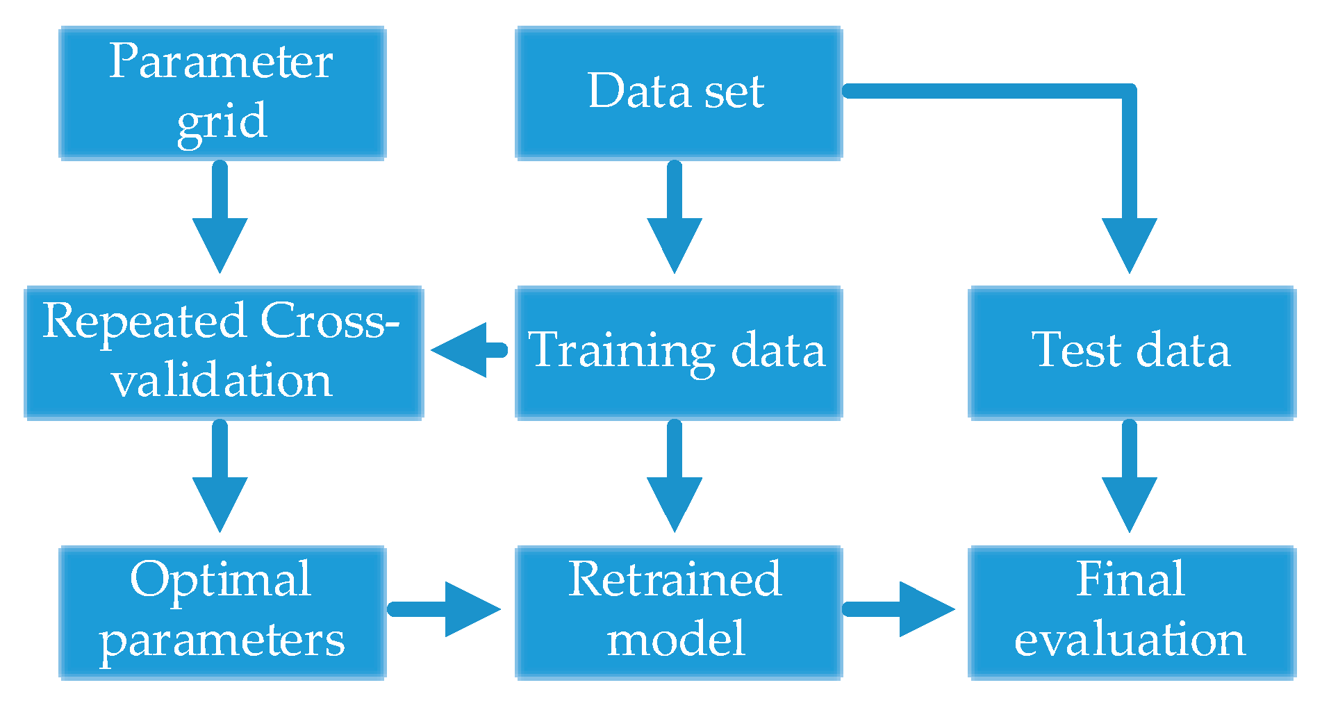
4.1.2. Parameter Selection Strategy
4.2. Results of the TEP Data
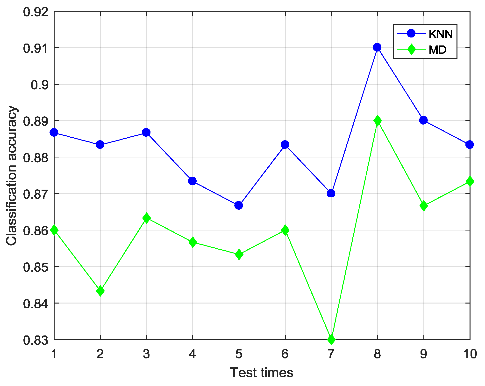
4.2.1. Selection of Classifier
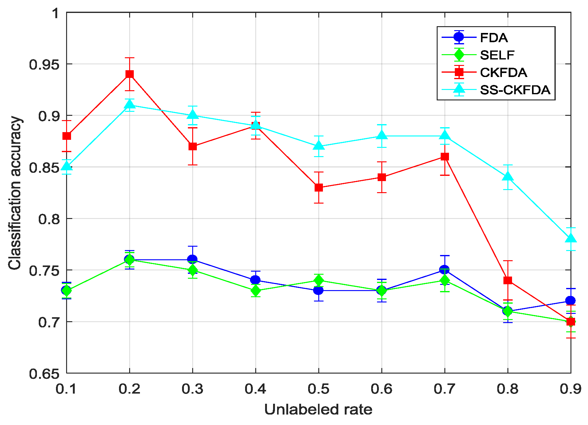
4.2.2. Results Comparison of SS-CKFDA with Other FDA Algorithms
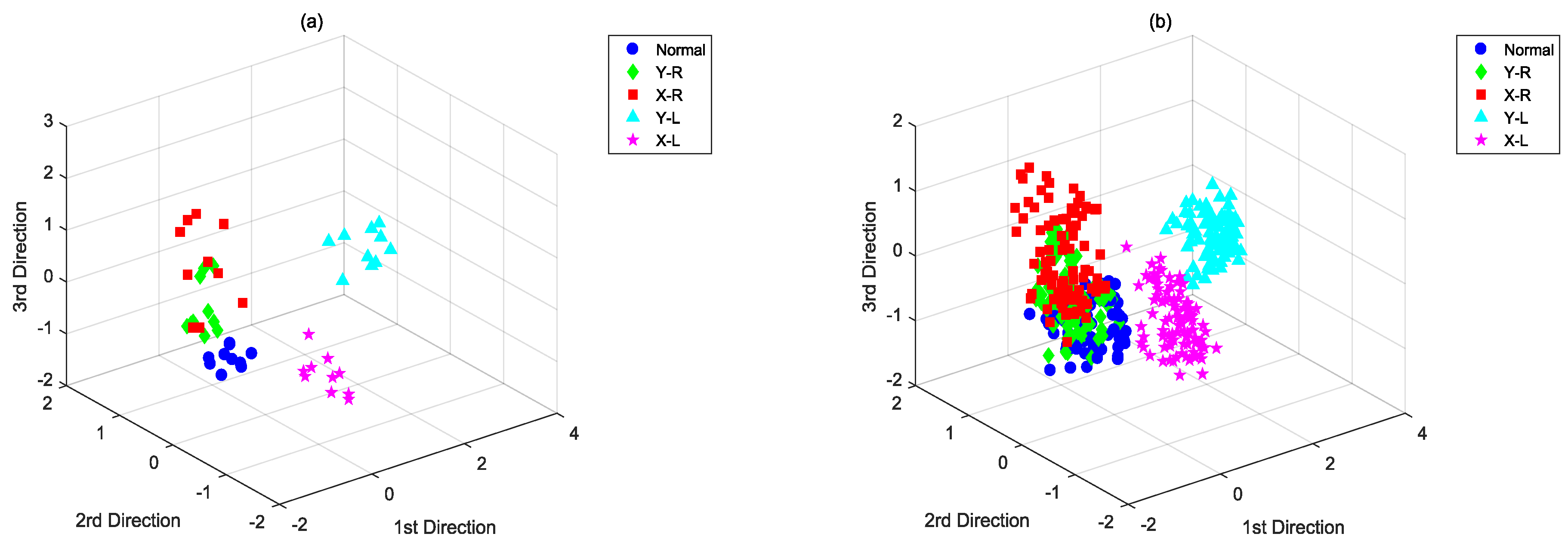
4.3. Results of the Automotive Assembly Process Data
5. Conclusions
Author Contributions
Acknowledgments
Conflicts of Interest
References
- Wang, H.; Chen, G.L.; Zhu, P.; Lin, Z.Q. Periodic trend detection from CMM data based on the continuous wavelet transform. Int. J. Adv. Manuf. Technol. 2006, 27, 733–737. [Google Scholar]
- Liu, Y.H.; Jin, S. Application of Bayesian networks for diagnostics in the assembly process by considering small measurement data sets. Int. J. Adv. Manuf. Technol. 2013, 65, 1229–1237. [Google Scholar] [CrossRef]
- Zhang, S.; Huang, P.S. Novel method for structured light system calibration. Opt. Eng. 2006, 45, 083601. [Google Scholar]
- Liu, T.; Yin, S.B.; Guo, Y.; Zhu, J.G. Rapid Global Calibration Technology for Hybrid Visual Inspection System. Sensors 2017, 17, 1440. [Google Scholar] [CrossRef] [PubMed]
- Jin, J.H.; Shi, J.J. State Space Modeling of Sheet Metal Assembly for Dimensional Control. J. Manuf. Sci. Eng. 1999, 121, 756–762. [Google Scholar] [CrossRef]
- Ding, Y.; Ceglarek, D.; Shi, J.J. Fault Diagnosis of Multistage Manufacturing Processes by Using State Space Approach. J. Manuf. Sci. Eng. 2002, 124, 313–322. [Google Scholar] [CrossRef] [Green Version]
- Jang, K.Y.; Yang, K. Improving Principal Component Analysis (PCA) in Automotive Body Assembly Using Artificial Neural Networks. J. Manuf. Syst. 2001, 20, 188–197. [Google Scholar] [CrossRef]
- Lian, J.; Lai, X.M.; Lin, Z.Q.; Yao, F.S. Application of data mining and process knowledge discovery in sheet metal assembly dimensional variation diagnosis. J. Mater. Process. Technol. 2002, 129, 315–320. [Google Scholar] [CrossRef]
- Chen, H.L.; Liu, D.Y.; Yang, B.; Liu, J.; Wang, G. A new hybrid method based on local fisher discriminant analysis and support vector machines for hepatitis disease diagnosis. Expert Syst. Appl. 2011, 38, 11796–11803. [Google Scholar] [CrossRef]
- Wen, T.L.; Yan, J.; Huang, D.Y.; Lu, K.; Deng, C.J.; Zeng, T.Y.; Yu, S.; He, Z.Y. Feature Extraction of Electronic Nose Signals Using QPSO-Based Multiple KFDA Signal Processing. Sensors 2018, 18, 388. [Google Scholar] [CrossRef] [PubMed]
- Portillo-Portillo, J.; Leyva, R.; Sanchez, V.; Sanchez-Perez, G.; Perez-Meana, H.; Olivares-Mercado, J.; Toscano-Medina, K.; Nakano-Miyatake, M. Cross View Gait Recognition Using Joint-Direct Linear Discriminant Analysis. Sensors 2017, 17, 6. [Google Scholar] [CrossRef] [PubMed]
- Liu, Z.L.; Qu, J.; Zuo, M.J.; Xu, H.B. Fault level diagnosis for planetary gearboxes using hybrid kernel feature selection and kernel Fisher discriminant analysis. Int. J. Adv. Manuf. Technol. 2013, 67, 1217–1230. [Google Scholar] [CrossRef]
- Chiang, L.H.; Russell, E.L.; Braatz, R.D. Fault diagnosis in chemical processes using Fisher discriminant analysis. Chemom. Intell. Lab. Syst. 2000, 50, 243–252. [Google Scholar] [CrossRef]
- Yang, J.; Frangi, A.F.; Yang, J.Y.; Zhang, D.; Jin, Z. KPCA plus LDA: A Complete Kernel Fisher Discriminant Framework for Feature Extraction and Recognition. IEEE Trans. Pattern Anal. Mach. Intell. 2005, 27, 230–244. [Google Scholar] [CrossRef] [PubMed] [Green Version]
- Schölkopf, B.; Smola, A.; Müller, K.R. Nonlinear Component Analysis as A Kernel Eigenvalue Problem. Neural Comput. 1998, 10, 1299–1319. [Google Scholar] [CrossRef]
- Cristianini, N.; Shawe-Taylor, J. An Introduction to Support Vector Machines and Other Kernel-Based Learning Methods; Cambridge University Press: Cambridge, UK, 2000. [Google Scholar]
- Sugiyama, M.; Idé, T.; Nakajima, S.; Sese, J. Semi-supervised local Fisher discriminant analysis for dimensionality reduction. Mach. Learn. 2010, 78, 35. [Google Scholar] [CrossRef]
- Zhu, X.; Goldberg, A.B. Introduction to semi-supervised learning. Synth. Lect. Artif. Intell. Mach. Learn. 2009, 3, 1–130. [Google Scholar] [CrossRef]
- Zhong, S.Y.; Wen, Q.J.; Ge, Z.Q. Semi-supervised Fisher discriminant analysis model for fault classification in industrial processes. Chemom. Intell. Lab. Syst. 2014, 138, 203–211. [Google Scholar] [CrossRef]
- Bishop, C.M. Pattern Recognition and Machine Learning; Springer: New York, NY, USA, 2006. [Google Scholar]
- Downs, J.J.; Vogel, E.F. A plant-wide industrial process control problem. Comput. Chem. Eng. 1993, 17, 245–255. [Google Scholar] [CrossRef]
- Leu, M.C.; Ji, Z. Non-Linear Displacement Sensor Based on Optical Triangulation Principle. U.S. Patent 5,113,080, 12 May 1992. [Google Scholar]
- Krstajic, D.; Buturovic, L.J.; Leahy, D.E.; Thomas, S. Cross-validation pitfalls when selecting and assessing regression and classification models. J. Cheminform. 2014, 6, 10. [Google Scholar] [CrossRef] [PubMed] [Green Version]
- Liu, J.T.; Chang, H.B.; Hsu, T.Y.; Ruan, X.Y. Prediction of the flow stress of high-speed steel during hot deformation using a BP artificial neural network. J. Mater. Process. Technol. 2000, 103, 200–205. [Google Scholar] [CrossRef]
- Chen, P.H.; Lin, C.J.; Schölkopf, B. A tutorial on ν-support vector machines. Appl. Stoch. Models Bus. Ind. 2005, 21, 111–136. [Google Scholar] [CrossRef]


| ID | Description | Type | Training Set | Test Set |
|---|---|---|---|---|
| 1 | No faulty | / | 500 | 100 |
| 2 | A/C feed ratio, B composition constant | Step change | 100 | 50 |
| 3 | B composition, A/C ration constant | Step change | 100 | 50 |
| 4 | A, B, C feed composition | Random variation | 100 | 50 |
| 5 | Condenser cooling water inlet temperature | Random variation | 100 | 50 |
| Min | Max | Average/Std | |
|---|---|---|---|
| SS-CKFDA + KNN | 0.87 | 0.91 | 0.883/0.012 |
| SS-CKFDA + MD | 0.83 | 0.89 | 0.859/0.016 |
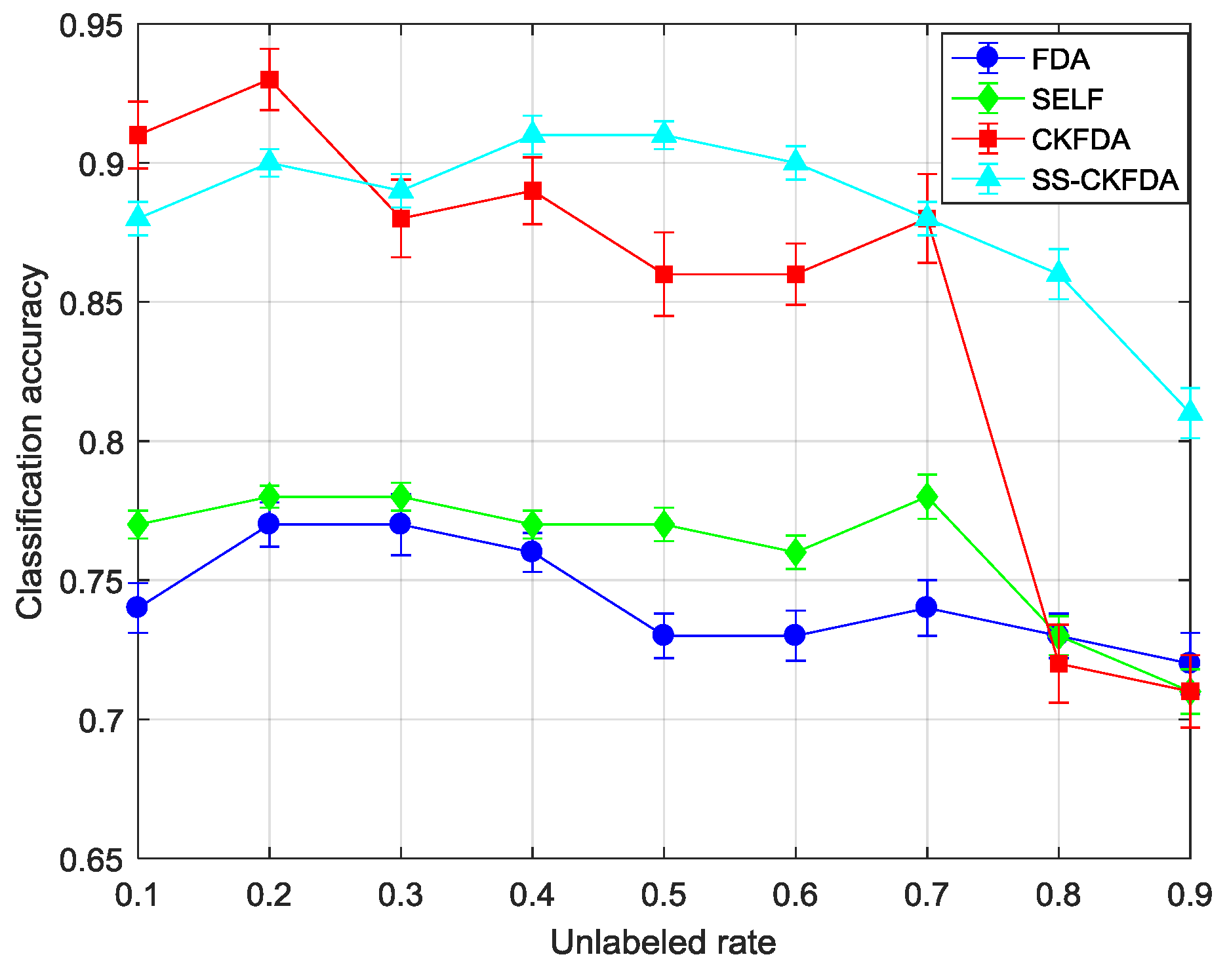
| Unlabeled Rate | FDA | SELF | CKFDA | SS-CKFDA | ||||
|---|---|---|---|---|---|---|---|---|
| Training Set | Test Set | Training Set | Test Set | Training Set | Test Set | Training Set | Test Set | |
| 10% | 0.74(0.009) | 0.73(0.008) | 0.77(0.005) | 0.73(0.007) | 0.91(0.012) | 0.88(0.015) | 0.88(0.006) | 0.85(0.007) |
| 20% | 0.77(0.008) | 0.76(0.009) | 0.78(0.004) | 0.76(0.007) | 0.93(0.011) | 0.94(0.016) | 0.9(0.005) | 0.91(0.006) |
| 30% | 0.77(0.011) | 0.76(0.013) | 0.78(0.005) | 0.75(0.008) | 0.88(0.014) | 0.87(0.018) | 0.89(0.006) | 0.90(0.009) |
| 40% | 0.76(0.007) | 0.74(0.009) | 0.77(0.005) | 0.73(0.006) | 0.89(0.012) | 0.89(0.013) | 0.91(0.007) | 0.89(0.009) |
| 50% | 0.73(0.008) | 0.73(0.01) | 0.77(0.006) | 0.74(0.006) | 0.86(0.015) | 0.83(0.015) | 0.91(0.005) | 0.87(0.01) |
| 60% | 0.73(0.009) | 0.73(0.011) | 0.76(0.006) | 0.73(0.008) | 0.86(0.011) | 0.84(0.015) | 0.9(0.006) | 0.88(0.011) |
| 70% | 0.74(0.01) | 0.75(0.014) | 0.78(0.008) | 0.74(0.011) | 0.88(0.016) | 0.86(0.018) | 0.88(0.006) | 0.88(0.008) |
| 80% | 0.73(0.008) | 0.71(0.011) | 0.73(0.007) | 0.71(0.008) | 0.72(0.014) | 0.74(0.019) | 0.86(0.009) | 0.84(0.012) |
| 90% | 0.72(0.011) | 0.72(0.012) | 0.71(0.008) | 0.70(0.01) | 0.71(0.013) | 0.70(0.016) | 0.81(0.009) | 0.78(0.011) |
| Average | 0.744(0.009) | 0.737(0.011) | 0.761(0.006) | 0.732(0.008) | 0.849(0.013) | 0.839(0.016) | 0.882(0.007) | 0.867(0.009) |
| FDA | SELF | CKFDA | SS-CKFDA | |||||
| Training Set | Test Set | Training Set | Test Set | Training Set | Test Set | Training Set | Test Set | |
| Normal | 0.34(0.135) | 0.26(0.012) | 0.42(0.147) | 0.34(0.011) | 0.78(0.148) | 0.68(0.015) | 0.88(0.103) | 0.72(0.008) |
| Y-R | 0.56(0.126) | 0.55(0.014) | 0.72(0.103) | 0.52(0.008) | 0.66(0.165) | 0.53(0.017) | 0.82(0.148) | 0.66(0.011) |
| X-R | 0.72(0.103) | 0.66(0.015) | 0.78(0.114) | 0.75(0.009) | 0.88(0.14) | 0.68(0.012) | 0.9(0.105) | 0.82(0.009) |
| Y-L | 1(0) | 1(0) | 1(0) | 0.98(0.006) | 1(0) | 1(0) | 1(0) | 1(0) |
| X-L | 1(0) | 0.95(0.011) | 1(0) | 0.95(0.005) | 1(0) | 0.95(0.006) | 1(0) | 0.98(0.003) |
| Average | 0.724(0.073) | 0.684(0.01) | 0.784(0.072) | 0.708(0.008) | 0.864(0.091) | 0.768(0.01) | 0.92(0.071) | 0.836(0.006) |
| BP-ANN | KNN | SVM | ||||||
| Training Set | Test Set | Training Set | Test Set | Training Set | Test Set | |||
| Normal | 0.32(0.103) | 0.35(0.022) | 0.48(0.169) | 0.53(0.028) | 0.9 (0.141) | 0.76(0.011) | ||
| Y-R | 0.66(0.135) | 0.65(0.025) | 0.62(0.148) | 0.56(0.025) | 0.72(0.193) | 0.62(0.014) | ||
| X-R | 0.9(0.105) | 0.84(0.018) | 0.68(0.235) | 0.72(0.031) | 0.86(0.165) | 0.74(0.008) | ||
| Y-L | 1(0) | 0.95(0.012) | 1(0) | 1(0) | 1(0) | 1(0) | ||
| X-L | 1(0) | 0.95(0.013) | 1(0) | 0.95(0.019) | 1(0) | 1(0) | ||
| Average | 0.776(0.069) | 0.748(0.018) | 0.756(0.11) | 0.752(0.021) | 0.896(0.1) | 0.824(0.007) | ||
| Average Training Time (ms) | |
|---|---|
| SS-CKFDA | 13.62 |
| CKFDA | 12.55 |
| SELF | 3.41 |
| FDA | 1.60 |
| BP-ANN | 265.54 |
| KNN | 142.36 |
| SVM | 21.78 |
© 2018 by the authors. Licensee MDPI, Basel, Switzerland. This article is an open access article distributed under the terms and conditions of the Creative Commons Attribution (CC BY) license (http://creativecommons.org/licenses/by/4.0/).
Share and Cite
Zeng, X.; Yin, S.-B.; Guo, Y.; Lin, J.-R.; Zhu, J.-G. A Novel Semi-Supervised Feature Extraction Method and Its Application in Automotive Assembly Fault Diagnosis Based on Vision Sensor Data. Sensors 2018, 18, 2545. https://doi.org/10.3390/s18082545
Zeng X, Yin S-B, Guo Y, Lin J-R, Zhu J-G. A Novel Semi-Supervised Feature Extraction Method and Its Application in Automotive Assembly Fault Diagnosis Based on Vision Sensor Data. Sensors. 2018; 18(8):2545. https://doi.org/10.3390/s18082545
Chicago/Turabian StyleZeng, Xuan, Shi-Bin Yin, Yin Guo, Jia-Rui Lin, and Ji-Gui Zhu. 2018. "A Novel Semi-Supervised Feature Extraction Method and Its Application in Automotive Assembly Fault Diagnosis Based on Vision Sensor Data" Sensors 18, no. 8: 2545. https://doi.org/10.3390/s18082545
APA StyleZeng, X., Yin, S.-B., Guo, Y., Lin, J.-R., & Zhu, J.-G. (2018). A Novel Semi-Supervised Feature Extraction Method and Its Application in Automotive Assembly Fault Diagnosis Based on Vision Sensor Data. Sensors, 18(8), 2545. https://doi.org/10.3390/s18082545