A Combined Deep Learning GRU-Autoencoder for the Early Detection of Respiratory Disease in Pigs Using Multiple Environmental Sensors


Abstract
:1. Introduction
- exchanging long short-term memory cells for GRU cells
- introducing particle swarm optimisation to optimise an anomaly detector that determines whether the loss from the GRU-AE is anomalous
- changing how the overall system is evaluated to demonstrate a more balanced anomaly detection system
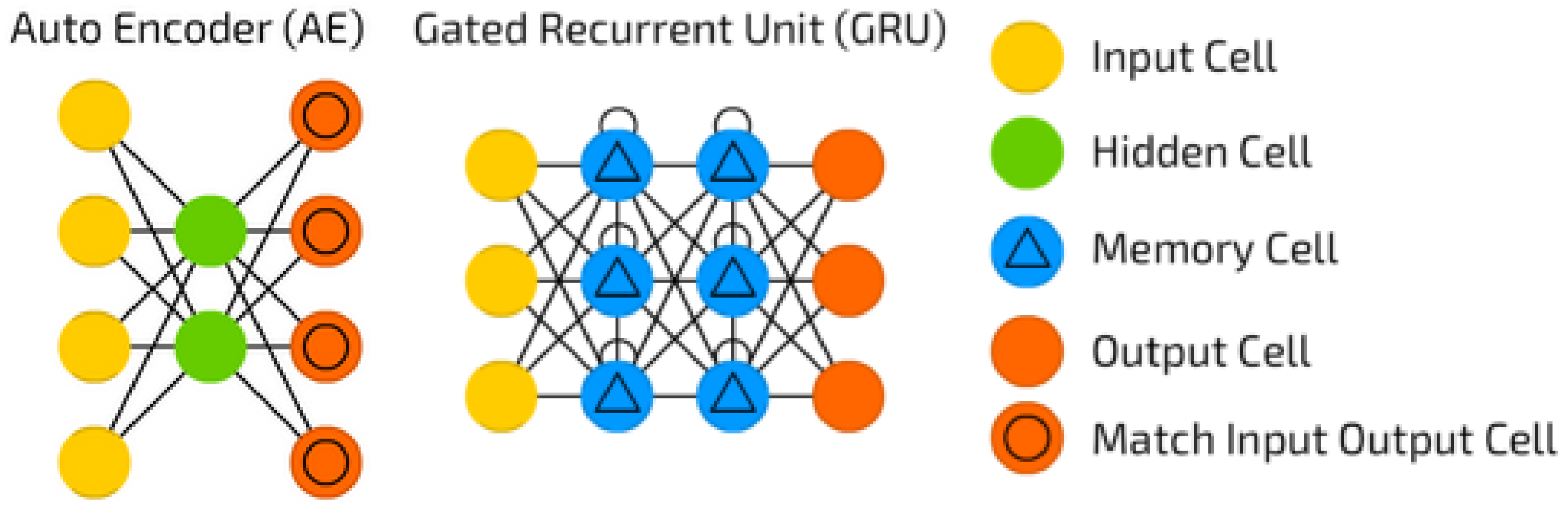
2. Background
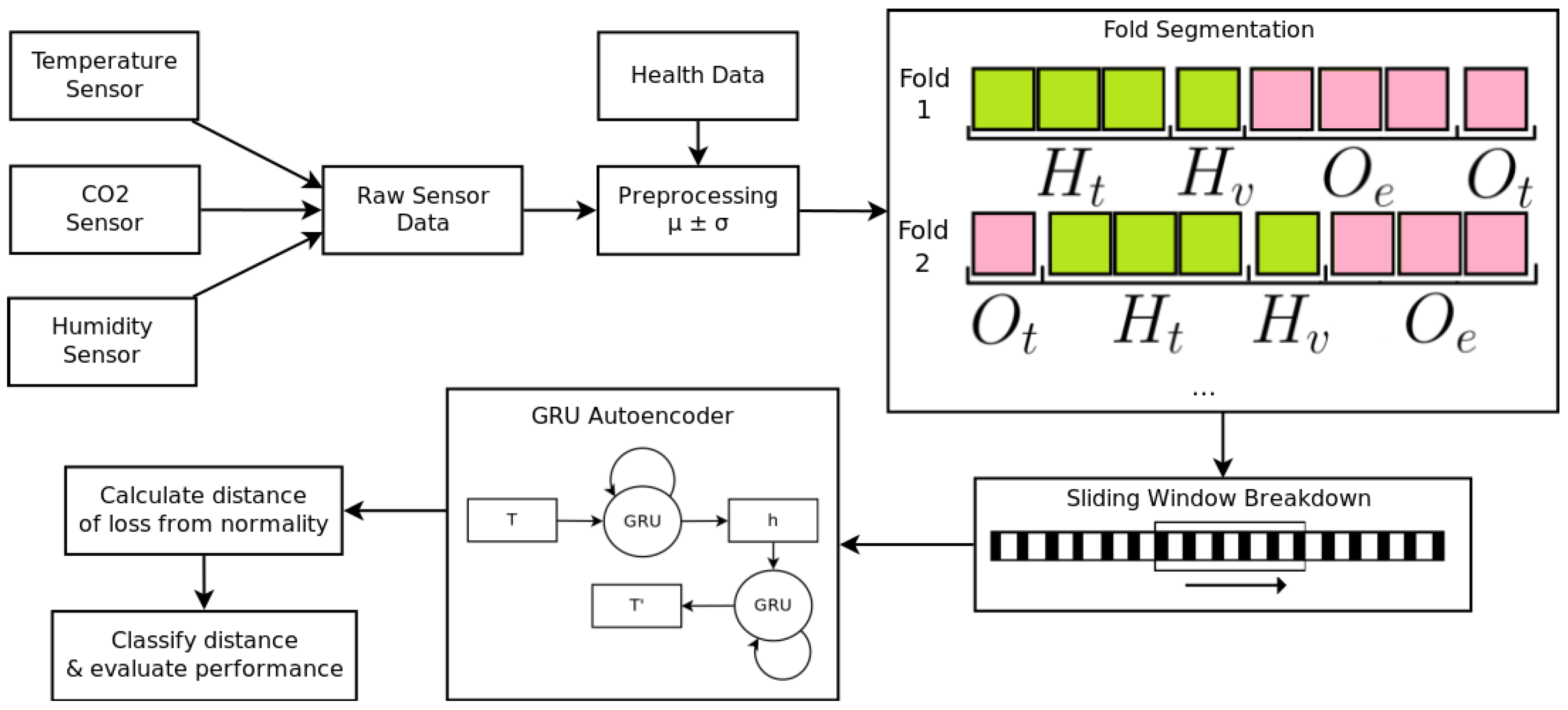
3. Experimental Design
3.1. Data Collection
3.2. Data Preprocessing
3.2.1. Separation of Assumed Healthy and Assumed Unhealthy Data
3.2.2. Splitting Data into Train, Validation, and Test Sets
3.2.3. Preliminary Experiments Utilising Batch Normalisation
4. Time-Series Early Warning Methods
4.1. GRU-Autoencoder
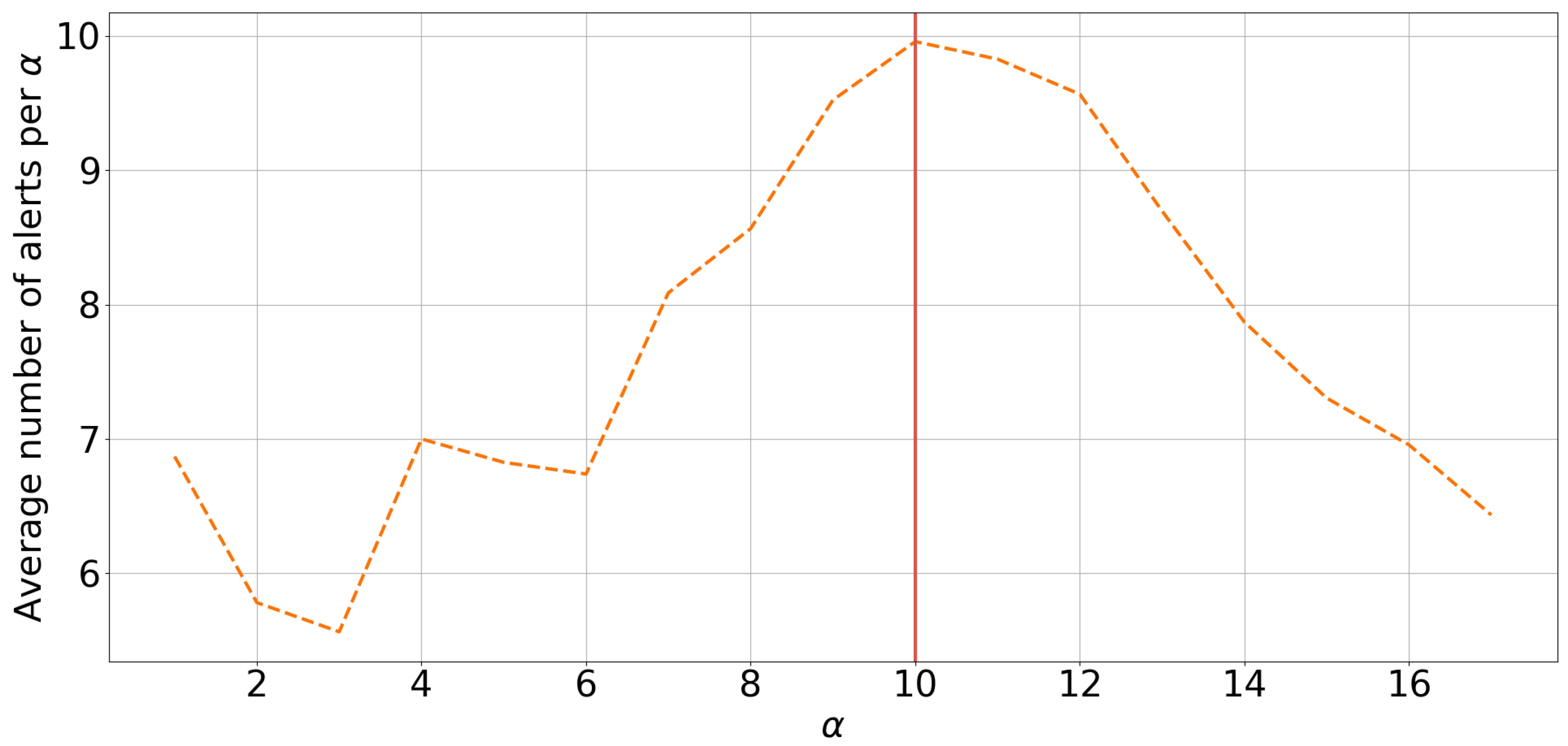
4.1.1. PSO-Optimised Anomaly Detection
4.2. Other Metrics Used for Evaluation
4.3. Methods Included for Comparison
4.3.1. Luminol
4.3.2. Time-Series Regression with Autoregression Integrated Moving Average (ARIMA)
4.3.3. Time-Series Regression with GRU Network (GRU-R)
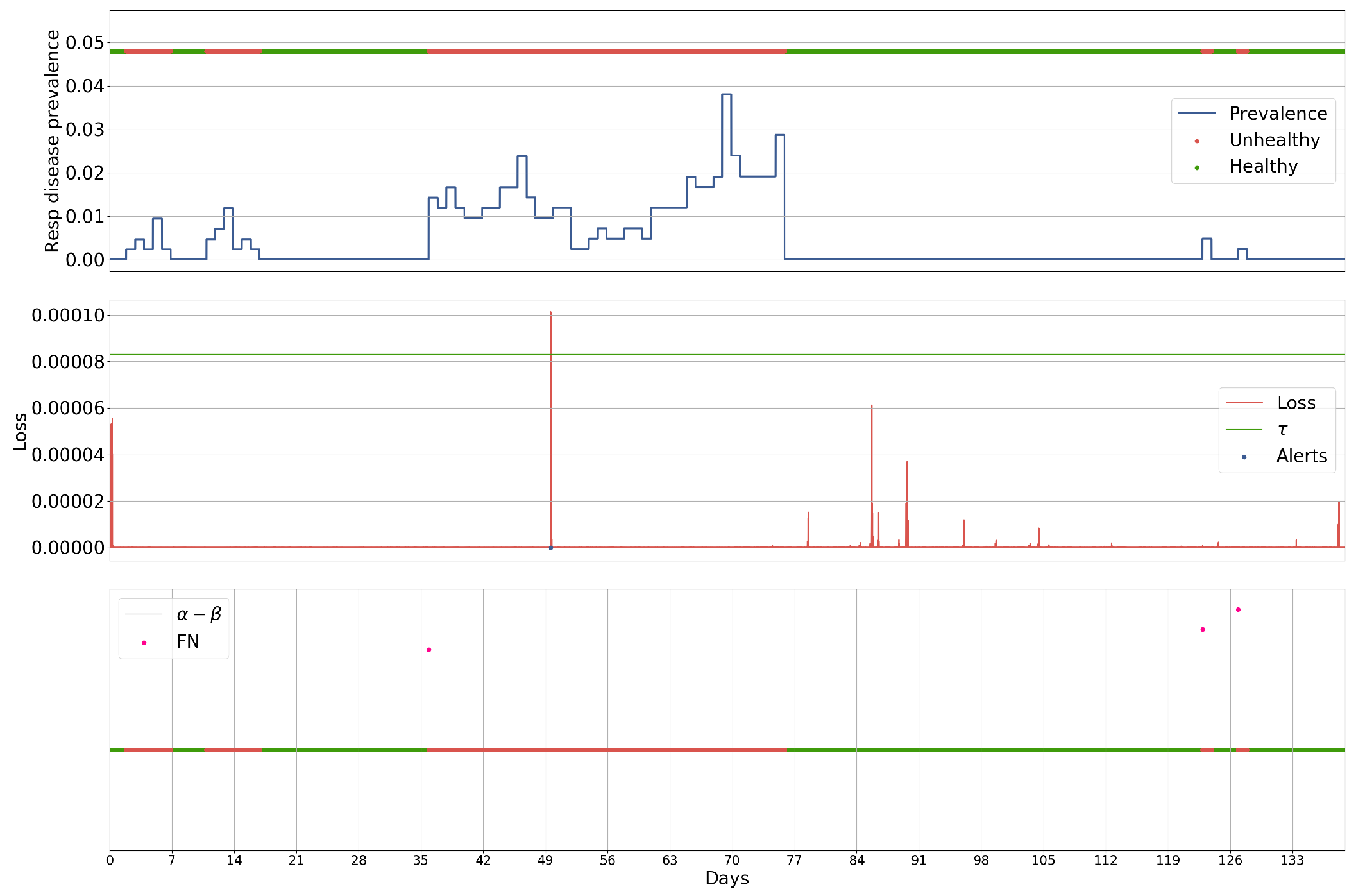
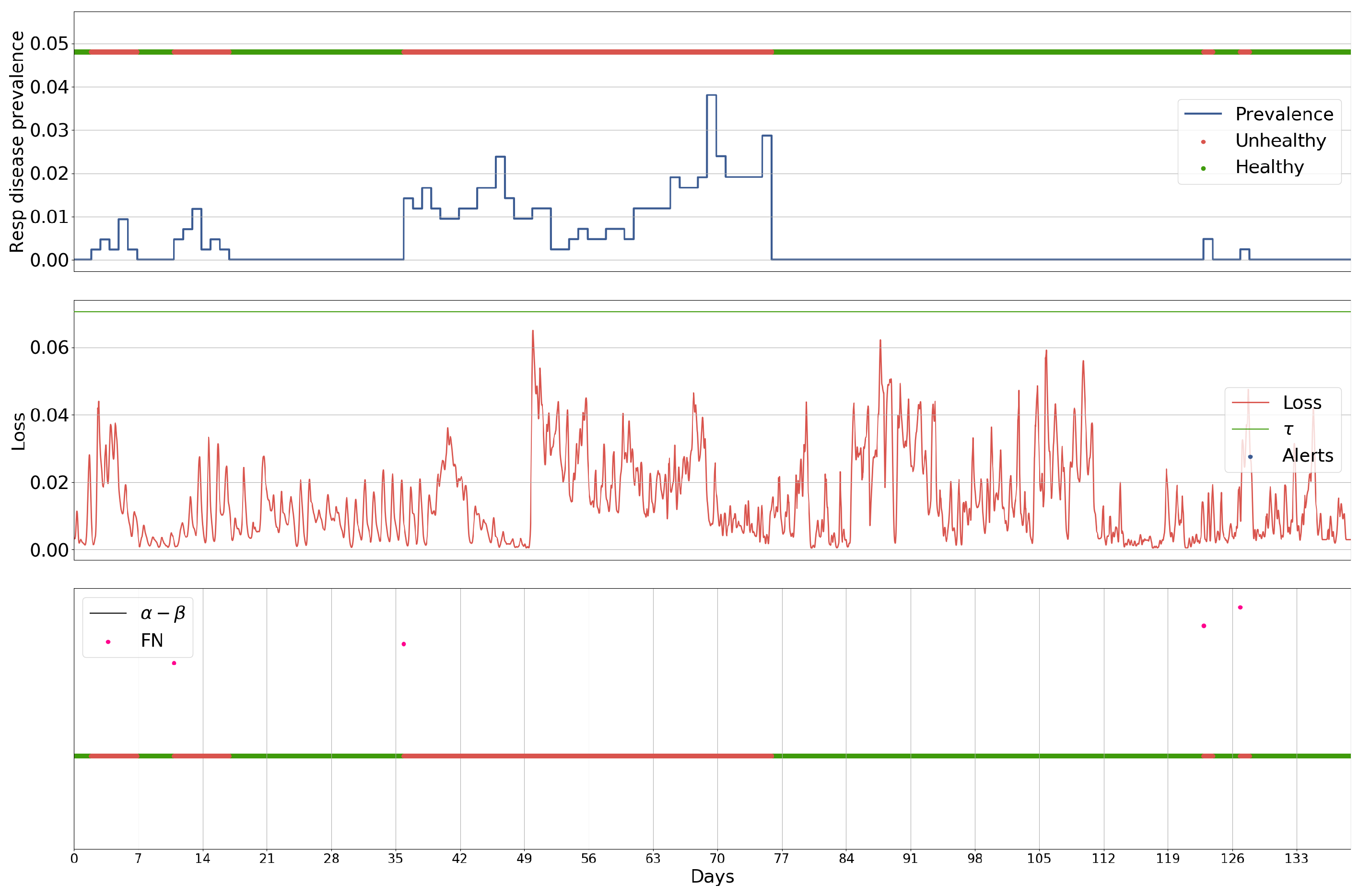
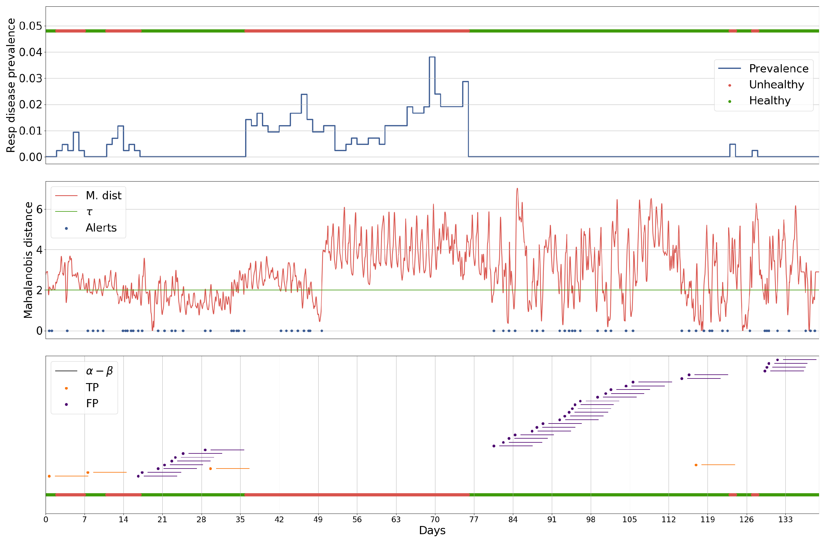
5. Results
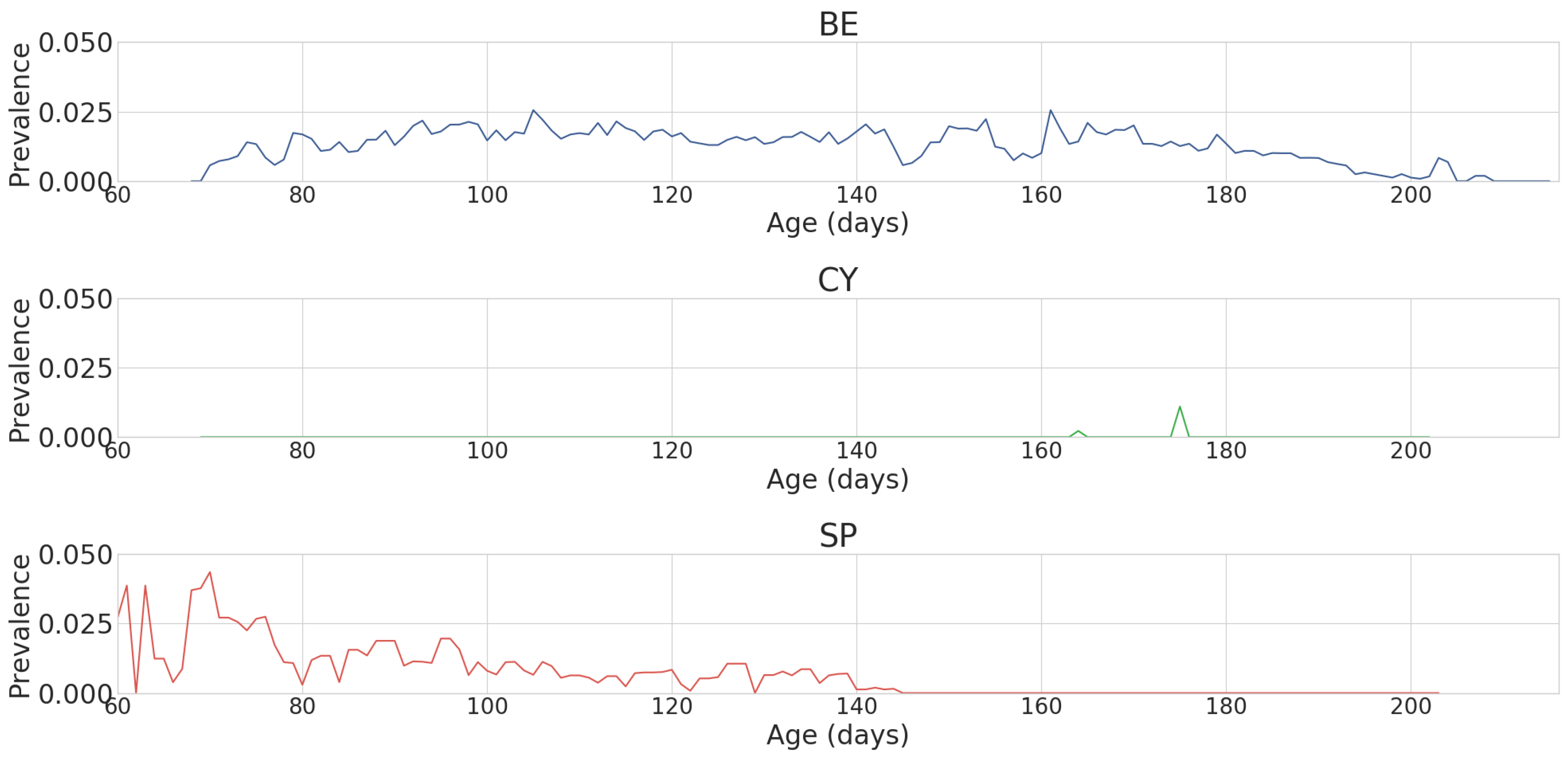
5.1. Case Study
5.2. Influence of the Number of Hidden Layers on GRU-AE Performance
5.3. Computation Time
6. Discussion
7. Conclusions
Author Contributions
Funding
Acknowledgments
Conflicts of Interest
References
- Huhn, R. Swine enzootic pneumonia: Incidence and effect on rate of body weight gain. Am. J. Vet. Res. 1970, 31, 1097–1108. [Google Scholar] [PubMed]
- Stärk, K.D. Epidemiological investigation of the influence of environmental risk factors on respiratory diseases in swine—A literature review. Vet. J. 2000, 159, 37–56. [Google Scholar] [CrossRef] [PubMed]
- Malhotra, P.; Ramakrishnan, A.; Anand, G.; Vig, L.; Agarwal, P.; Shroff, G. LSTM-based Encoder-Decoder for Multi-sensor Anomaly Detection. Available online: https://arxiv.org/abs/1607.00148 (accessed on 20 June 2018).
- Malhotra, P.; Vig, L.; Shroff, G.; Agarwal, P. Long short term memory networks for anomaly detection in time series. In Proceedings; Presses Universitaires de Louvain: Louvain-la-Neuve, Belgium, 2015; p. 89. [Google Scholar]
- Morales, I.R.; Cebrián, D.R.; Blanco, E.F.; Sierra, A.P. Early warning in egg production curves from commercial hens: A SVM approach. Comput. Electron. Agric. 2016, 121, 169–179. [Google Scholar] [CrossRef]
- Singh, R.K.; Sharma, V.C. Ensemble Approach for Zoonotic Disease Prediction Using Machine Learning Techniques; Indian Institute of Management: Ahmedabad, India, 2015. [Google Scholar]
- Valdes-Donoso, P.; VanderWaal, K.; Jarvis, L.S.; Wayne, S.R.; Perez, A.M. Using Machine learning to Predict swine Movements within a regional Program to improve control of infectious Diseases in the US. Front. Vet. Sci. 2017, 4, 2. [Google Scholar] [CrossRef] [PubMed]
- Cabral, G.G.; de Oliveira, A.L.I. One-class Classification for heart disease diagnosis. In Proceedings of the IEEE International Conference on Systems, Man and Cybernetics (SMC), San Diego, CA, USA, 5–8 October 2014; pp. 2551–2556. [Google Scholar]
- Leng, Q.; Qi, H.; Miao, J.; Zhu, W.; Su, G. One-class classification with extreme learning machine. Math. Probl. Eng. 2015, 2015. [Google Scholar] [CrossRef]
- Thompson, R.; Matheson, S.M.; Plötz, T.; Edwards, S.A.; Kyriazakis, I. Porcine lie detectors: Automatic quantification of posture state and transitions in sows using inertial sensors. Comput. Electron. Agric. 2016, 127, 521–530. [Google Scholar] [CrossRef] [PubMed]
- Münz, G.; Li, S.; Carle, G. Traffic anomaly detection using k-means clustering. In GI/ITG Workshop MMBnet; University of Hamburg: Hamburg, Germany, 2017; pp. 13–14. [Google Scholar]
- Ambusaidi, M.A.; Tan, Z.; He, X.; Nanda, P.; Lu, L.F.; Jamdagni, A. Intrusion detection method based on nonlinear correlation measure. Int. J. Internet Protoc. Technol. 2014, 8, 77–86. [Google Scholar] [CrossRef]
- Aghabozorgi, S.; Shirkhorshidi, A.S.; Wah, T.Y. Time-series clustering—A decade review. Inf. Syst. 2015, 53, 16–38. [Google Scholar] [CrossRef]
- Wong, W.K.; Moore, A.W.; Cooper, G.F.; Wagner, M.M. Bayesian network anomaly pattern detection for disease outbreaks. In Proceedings of the 20th International Conference on Machine Learning (ICML-03), Washington, DC, USA, 21–24 August 2003; pp. 808–815. [Google Scholar]
- Wong, W.K.; Moore, A.; Cooper, G.; Wagner, M. What’s strange about recent events (WSARE): An algorithm for the early detection of disease outbreaks. J. Mach. Learn. Res. 2005, 6, 1961–1998. [Google Scholar]
- Chauhan, S.; Vig, L. Anomaly detection in ECG time signals via deep long short-term memory networks. In Proceedings of the IEEE International Conference on Data Science and Advanced Analytics (DSAA), Paris, France, 19–21 October 2015; pp. 1–7. [Google Scholar]
- Haque, S.A.; Rahman, M.; Aziz, S.M. Sensor anomaly detection in wireless sensor networks for healthcare. Sensors 2015, 15, 8764–8786. [Google Scholar] [CrossRef] [PubMed]
- Veeravalli, B.; Deepu, C.J.; Ngo, D. Real-Time, Personalized Anomaly Detection in Streaming Data for Wearable Healthcare Devices. In Handbook of Large-Scale Distributed Computing in Smart Healthcare; Springer: Berlin, Germany, 2017; pp. 403–426. [Google Scholar]
- Kanarachos, S.; Mathew, J.; Chroneos, A.; Fitzpatrick, M. Anomaly detection in time series data using a combination of wavelets, neural networks and Hilbert transform. In Proceedings of the 6th IEEE International Conference on Information, Intelligence, Systems and Applications (IISA2015), Corfu, Greece, 6–8 July 2015; pp. 1–6. [Google Scholar]
- Li, J.; Pedrycz, W.; Jamal, I. Multivariate time series anomaly detection: A framework of Hidden Markov Models. Appl. Soft Comput. 2017, 60, 229–240. [Google Scholar] [CrossRef]
- Chuah, M.C.; Fu, F. ECG anomaly detection via time series analysis. In Proceedings of the International Symposium on Parallel and Distributed Processing and Applications, Niagara Falls, ON, Canada, 28 August–1 September 2007; pp. 123–135. [Google Scholar]
- Chen, X.W.; Lin, X. Big data deep learning: Challenges and perspectives. IEEE Access 2014, 2, 514–525. [Google Scholar] [CrossRef]
- Kamilaris, A.; Prenafeta-Boldú, F.X. Deep learning in agriculture: A survey. Comput. Electron. Agric. 2018, 147, 70–90. [Google Scholar] [CrossRef]
- Veen, F.V. A Mostly complete chart of Neural Networks; The Asimov Institute: Utrecht, The Netherlands, 2016. [Google Scholar]
- Lv, Y.; Duan, Y.; Kang, W.; Li, Z.; Wang, F.Y. Traffic flow prediction with big data: A deep learning approach. IEEE Trans. Intell. Transp. Syst. 2015, 16, 865–873. [Google Scholar] [CrossRef]
- Andrews, J.T.; Morton, E.J.; Griffin, L.D. Detecting anomalous data using auto-encoders. Int. J. Mach. Learn. Comput. 2016, 6, 21. [Google Scholar]
- Rahman, A.; Smith, D.; Hills, J.; Bishop-Hurley, G.; Henry, D.; Rawnsley, R. A comparison of autoencoder and statistical features for cattle behaviour classification. In Proceedings of the International Joint Conference on Neural Networks (IJCNN), Vancouver, BC, Canada, 24–29 July 2016; pp. 2954–2960. [Google Scholar]
- Al Moubayed, N.; Breckon, T.; Matthews, P.; McGough, A.S. Sms spam filtering using probabilistic topic modelling and stacked denoising autoencoder. In Proceedings of the International Conference on Artificial Neural Networks, Barcelona, Spain, 6–9 September 2016; pp. 423–430. [Google Scholar]
- Zoetis. Individual Pig Care; Zoetis: Parsippany-Troy Hills, NJ, USA, 2012. [Google Scholar]
- Alert, G. Application Areas. Available online: http://www.general-alert.com/Applications (accessed on 30 April 2018).
- Whittemore, C.T.; Kyriazakis, I. Whittemore’s Science and Practice of Pig Production; John Wiley & Sons: Hoboken, NJ, USA, 2006. [Google Scholar]
- The World Organisation for Animal Health. Infection With Porcine Reproductive and Respiratory Syndrome Virus; The World Organisation for Animal Health: Paris, France, 2014. [Google Scholar]
- Ioffe, S.; Szegedy, C. Batch normalization: Accelerating deep network training by reducing internal covariate shift. arXiv 2015, preprint. arXiv:1502.03167. [Google Scholar]
- Sutskever, I.; Vinyals, O.; Le, Q.V. Sequence to sequence learning with neural networks. In Advances in Neural Information Processing Systems; Curran Associates, Inc.: New York, NY, USA, 2014; pp. 3104–3112. [Google Scholar]
- Tieleman, T.; Hinton, G. Lecture 6.5-rmsprop: Divide the gradient by a running average of its recent magnitude. COURSERA Neural Netw. Mach. Learn. 2012, 4, 26–31. [Google Scholar]
- Cleveland, W.S. Robust locally weighted regression and smoothing scatterplots. J. Am. Stat. Assoc. 1979, 74, 829–836. [Google Scholar] [CrossRef]
- Shi, Y.; Eberhart, R. A modified particle swarm optimizer. In Proceedings of the IEEE International Conference on Evolutionary Computation Proceedings, IEEE World Congress on Computational Intelligence, Anchorage, AK, USA, 4–9 May 1998; pp. 69–73. [Google Scholar]
- Holm, S. A simple sequentially rejective multiple test procedure. Scand. J. Stat. 1979, 6, 65–70. [Google Scholar]
- LinkedIn. Luminol. 2016. Available online: https://github.com/linkedin/luminol (accessed on 30 April 2018).
- Lin, J.; Keogh, E.; Wei, L.; Lonardi, S. Experiencing SAX: A novel symbolic representation of time series. Data Min. Knowl. Discov. 2007, 15, 107–144. [Google Scholar] [CrossRef]
- Wei, L.; Kumar, N.; Lolla, V.N.; Keogh, E.J.; Lonardi, S.; Ratanamahatana, C.A. Assumption-Free Anomaly Detection in Time Series. In Proceedings of the International Conference on Scientific and Statistical Database Management, La Jolla, CA, USA, 29 June–1 July 2005; Volume 5, pp. 237–242. [Google Scholar]
- Mortensen, S.; Stryhn, H.; Søgaard, R.; Boklund, A.; Stärk, K.D.; Christensen, J.; Willeberg, P. Risk factors for infection of sow herds with porcine reproductive and respiratory syndrome (PRRS) virus. Prev. Vet. Med. 2002, 53, 83–101. [Google Scholar] [CrossRef]
- Chung, J.; Gulcehre, C.; Cho, K.; Bengio, Y. Empirical evaluation of gated recurrent neural networks on sequence modeling. Available online: https://arxiv.org/abs/1412.3555 (accessed on 12 February 2018).
- Chung, J.; Gulcehre, C.; Cho, K.; Bengio, Y. Gated feedback recurrent neural networks. In Proceedings of the International Conference on Machine Learning, Lille, France, 6–11 July 2015; pp. 2067–2075. [Google Scholar]
- Karpathy, A.; Johnson, J.; Li, F.-F. Visualizing and understanding recurrent networks. Available online: https://arxiv.org/abs/1506.02078 (accessed on 17 March 2018).
- Jozefowicz, R.; Zaremba, W.; Sutskever, I. An empirical exploration of recurrent network architectures. In Proceedings of the International Conference on Machine Learning, Lille, France, 6–11 July 2015; pp. 2342–2350. [Google Scholar]
- Berckmans, D. Precision livestock farming technologies for welfare management in intensive livestock systems. Sci. Tech. Re. Off. Int. Epizoot. 2014, 33, 189–196. [Google Scholar] [CrossRef]
- Matthews, S.G.; Miller, A.L.; Clapp, J.; Plötz, T.; Kyriazakis, I. Early detection of health and welfare compromises through automated detection of behavioural changes in pigs. Vet. J. 2016, 217, 43–51. [Google Scholar] [CrossRef] [PubMed]
- Chung, Y.; Oh, S.; Lee, J.; Park, D.; Chang, H.H.; Kim, S. Automatic detection and recognition of pig wasting diseases using sound data in audio surveillance systems. Sensors 2013, 13, 12929–12942. [Google Scholar] [CrossRef] [PubMed]
- Krakovna, V.; Doshi-Velez, F. Increasing the interpretability of recurrent neural networks using hidden Markov models. Available online: https://arxiv.org/abs/1606.05320v2 (accessed on 29 December 2017).
- Samek, W.; Wiegand, T.; Müller, K.R. Explainable Artificial Intelligence: Understanding, Visualizing and Interpreting Deep Learning Models. Available online: https://arxiv.org/abs/1708.08296 (accessed on 23 March 2018).


| Hyper-Parameter | Value |
|---|---|
| Hidden size | 4 |
| No of layers | 20 |
| Mini-batch size | 1024 |
| Dropout | 0.5 |
| Learning rate | |
| Momentum | 0.3 |
| ID | Events | Luminol | ARIMA | GRU-R | GRU-AE | ||||||||
|---|---|---|---|---|---|---|---|---|---|---|---|---|---|
| P | R | MCC | P | R | MCC | P | R | MCC | P | R | MCC | ||
| 5 | 0 | 0.111 | 0.125 | 0.118 | 1.0 | 1.0 | 1.0 | 1.0 | 1.0 | 1.0 | 0.0 | 0.0 | 0.0 |
| 9 | 0 | 1.0 | 0.1 | 0.316 | 1.0 | 1.0 | 1.0 | 1.0 | 1.0 | 1.0 | 1.0 | 1.0 | 1.0 |
| 10 | 0 | 0.0 | 0.0 | 0.0 | 1.0 | 1.0 | 1.0 | 0.0 | 0.0 | 0.0 | 1.0 | 1.0 | 1.0 |
| 14 | 0 | 1.0 | 1.0 | 1.0 | 1.0 | 1.0 | 1.0 | 1.0 | 1.0 | 1.0 | 1.0 | 1.0 | 1.0 |
| 16 | 0 | 1.0 | 1.0 | 1.0 | 0.0 | 1.0 | 0.0 | 1.0 | 1.0 | 1.0 | 1.0 | 1.0 | 1.0 |
| 17 | 0 | 1.0 | 0.667 | 0.816 | 1.0 | 1.0 | 1.0 | 1.0 | 1.0 | 1.0 | 1.0 | 1.0 | 1.0 |
| 18 | 0 | 1.0 | 1.0 | 1.0 | 0.0 | 1.0 | 0.0 | 1.0 | 1.0 | 1.0 | 1.0 | 1.0 | 1.0 |
| 19 | 0 | 1.0 | 0.667 | 0.816 | 1.0 | 1.0 | 1.0 | 1.0 | 1.0 | 1.0 | 1.0 | 1.0 | 1.0 |
| 24 | 0 | 1.0 | 1.0 | 1.0 | 1.0 | 1.0 | 1.0 | 1.0 | 1.0 | 1.0 | 1.0 | 1.0 | 1.0 |
| 26 | 4 | 1.0 | 0.667 | 0.816 | 0.053 | 0.5 | 0.162 | 1.0 | 0.0 | 0.0 | 0.250 | 1.0 | 0.500 |
| 27 | 5 | 0.0 | 0.0 | 0.0 | 1.0 | 0.0 | 0.0 | 0.0 | 0.0 | 0.0 | 0.111 | 1.0 | 0.333 |
| 28 | 3 | 0.0 | 0.0 | 0.0 | 1.0 | 0.0 | 0.0 | 0.0 | 0.0 | 0.0 | 1.0 | 1.0 | 1.0 |
| 29 | 1 | 0.0 | 0.0 | 0.0 | 1.0 | 1.0 | 1.0 | 0.0 | 0.0 | 0.0 | 1.0 | 1.0 | 0.0 |
| 30 | 0 | 0.0 | 0.0 | 0.0 | 0.0 | 1.0 | 0.0 | 1.0 | 1.0 | 1.0 | 1.0 | 1.0 | 1.0 |
| 31 | 1 | 0.0 | 0.0 | 0.0 | 1.0 | 1.0 | 1.0 | 1.0 | 1.0 | 1.0 | 0.050 | 1.0 | 0.224 |
| 32 | 0 | 0.0 | 0.0 | 0.0 | 1.0 | 1.0 | 1.0 | 1.0 | 1.0 | 1.0 | 1.0 | 1.0 | 1.0 |
| Avg. Events = 0 | 0.647 | 0.505 | 0.551 | 0.727 | 1.000 | 0.727 | 0.909 | 0.909 | 0.909 | 0.909 | 0.909 | 0.909 | |
| Avg. Events > 0 | 0.200 | 0.133 | 0.163 | 0.811 | 0.500 | 0.432 | 0.400 | 0.400 | 0.200 | 0.482 | 1.000 | 0.411 | |
| Avg. All | 0.507 | 0.390 | 0.430 | 0.753 | 0.844 | 0.635 | 0.750 | 0.688 | 0.688 | 0.776 | 0.938 | 0.754 | |
| I/B/C | 7/5/4 | 5/1/10 | 5/0/11 | 2/3/11 | |||||||||
| ID | Events | Luminol | ARIMA | GRU-R | GRU-AE | ||||
|---|---|---|---|---|---|---|---|---|---|
| 5 | 0 | 12 | 4 | 12 | 1 | 1 | 6 | 1 | 1 |
| 9 | 0 | 12 | 4 | 12 | 1 | 1 | 6 | 1 | 2 |
| 10 | 0 | 12 | 4 | 12 | 1 | 1 | 6 | 1 | 2 |
| 14 | 0 | 12 | 4 | 12 | 1 | 1 | 6 | 1 | 4 |
| 16 | 0 | 12 | 4 | 12 | 1 | 1 | 6 | 3 | 1 |
| 17 | 0 | 12 | 4 | 12 | 1 | 1 | 6 | 1 | 5 |
| 18 | 0 | 12 | 4 | 12 | 1 | 1 | 6 | 3 | 5 |
| 19 | 0 | 12 | 4 | 12 | 1 | 1 | 6 | 1 | 5 |
| 24 | 0 | 12 | 4 | 12 | 1 | 1 | 6 | 1 | 6 |
| 26 | 4 | 12 | 4 | 12 | 1 | 2 | 6 | 3 | 6 |
| 27 | 5 | 12 | 4 | 12 | 4 | 4 | 6 | 1 | 6 |
| 28 | 3 | 12 | 4 | 12 | 1 | 5 | 6 | 8 | 6 |
| 29 | 1 | 12 | 4 | 12 | 2 | 1 | 6 | 2 | 6 |
| 30 | 0 | 12 | 4 | 12 | 1 | 1 | 6 | 4 | 6 |
| 31 | 1 | 12 | 4 | 12 | 1 | 1 | 6 | 1 | 6 |
| 32 | 0 | 12 | 4 | 12 | 1 | 1 | 6 | 8 | 5 |
© 2018 by the authors. Licensee MDPI, Basel, Switzerland. This article is an open access article distributed under the terms and conditions of the Creative Commons Attribution (CC BY) license (http://creativecommons.org/licenses/by/4.0/).
Share and Cite
Cowton, J.; Kyriazakis, I.; Plötz, T.; Bacardit, J. A Combined Deep Learning GRU-Autoencoder for the Early Detection of Respiratory Disease in Pigs Using Multiple Environmental Sensors. Sensors 2018, 18, 2521. https://doi.org/10.3390/s18082521
Cowton J, Kyriazakis I, Plötz T, Bacardit J. A Combined Deep Learning GRU-Autoencoder for the Early Detection of Respiratory Disease in Pigs Using Multiple Environmental Sensors. Sensors. 2018; 18(8):2521. https://doi.org/10.3390/s18082521
Chicago/Turabian StyleCowton, Jake, Ilias Kyriazakis, Thomas Plötz, and Jaume Bacardit. 2018. "A Combined Deep Learning GRU-Autoencoder for the Early Detection of Respiratory Disease in Pigs Using Multiple Environmental Sensors" Sensors 18, no. 8: 2521. https://doi.org/10.3390/s18082521
APA StyleCowton, J., Kyriazakis, I., Plötz, T., & Bacardit, J. (2018). A Combined Deep Learning GRU-Autoencoder for the Early Detection of Respiratory Disease in Pigs Using Multiple Environmental Sensors. Sensors, 18(8), 2521. https://doi.org/10.3390/s18082521