Health Management Decision of Sensor System Based on Health Reliability Degree and Grey Group Decision-Making


Abstract
1. Introduction
- (1)
- (2)
- Take high redundancy gas sensor array for data acquisition to minimize the impact of fault sensor on the detection and analysis effect of pattern recognition methods subsequently [4].
- (3)
2. Health Management Decision
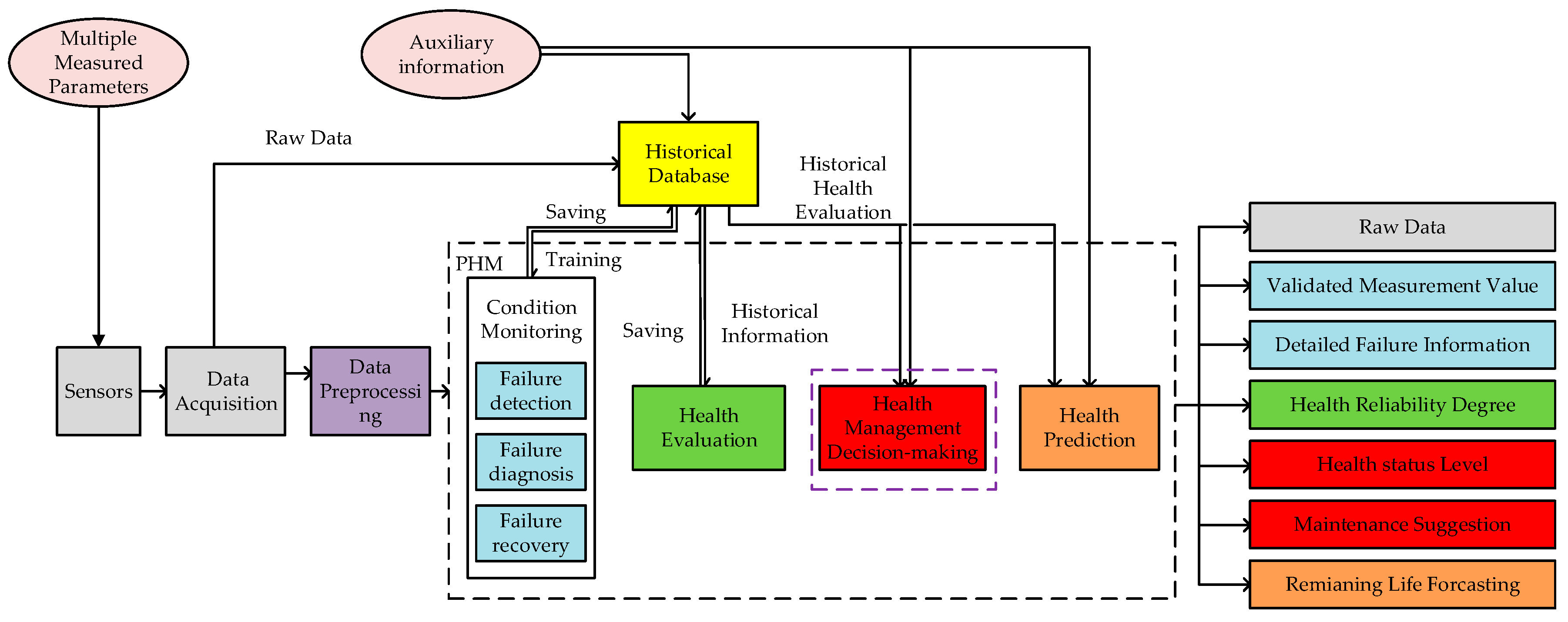
2.1. Implementation Framework of Health Management and Maintenance Decision
- Health: The whole system is very healthy. All of the sensors are also healthy. Their measurements are close to the expected value. There is no need to repair the system.
- Subhealth: The system is working at subhealthy status. The output of the system is within a normal range. All of the parameters may fluctuate near their expected value. It is essential to execute preventive maintenance regularly. Failure detection and failure isolation methods should be used in this situation.
- Failure Edge: The system is nearly failure. Their actual measurements have deviated from the expected value, but they have not deviated completely. In this status some sensors may be faulty, but the system can work effectively when fault recovery is performed. Corrective maintenance is needed after experiment [25]. Failure recovery method will be applied in this status to improve the work status sometimes.
- Failure: The system is failure. Most of sensors are failure. The actual output has completely deviated from its expected results. Immediate repaired the failure components or replacement failure components immediately may be the best choice.
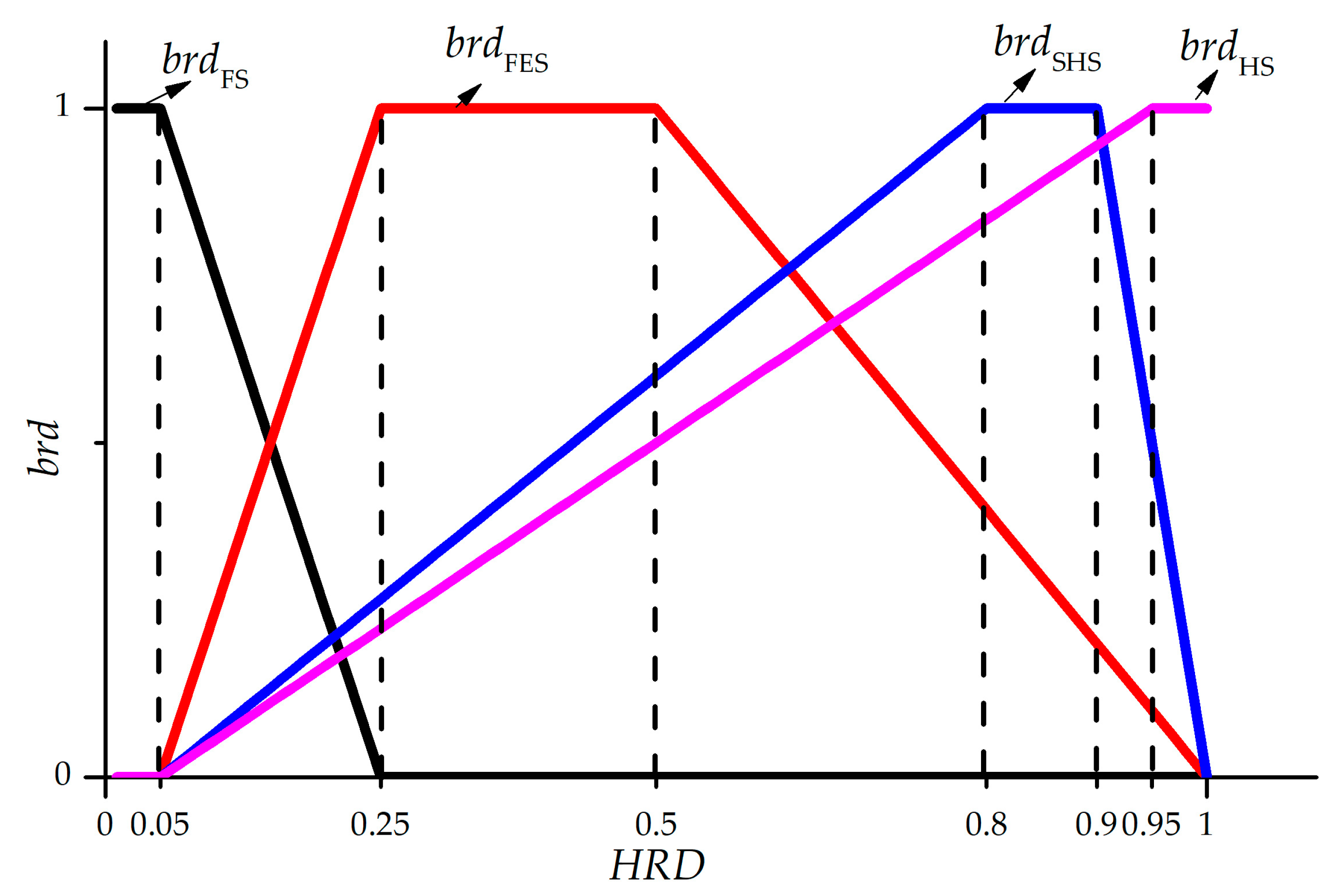
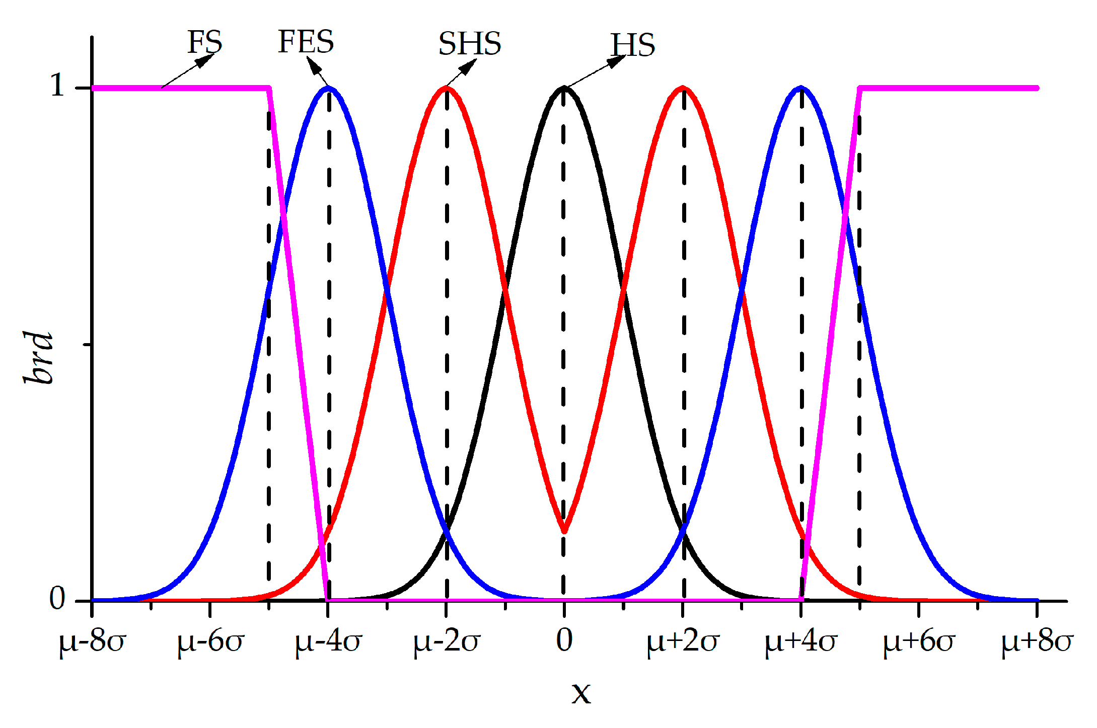
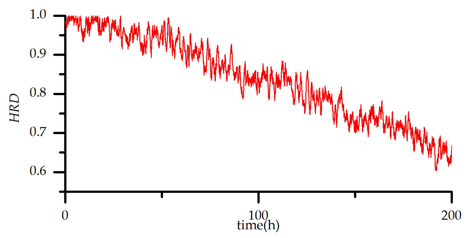
2.2. Health Reliability Degree (HRD)
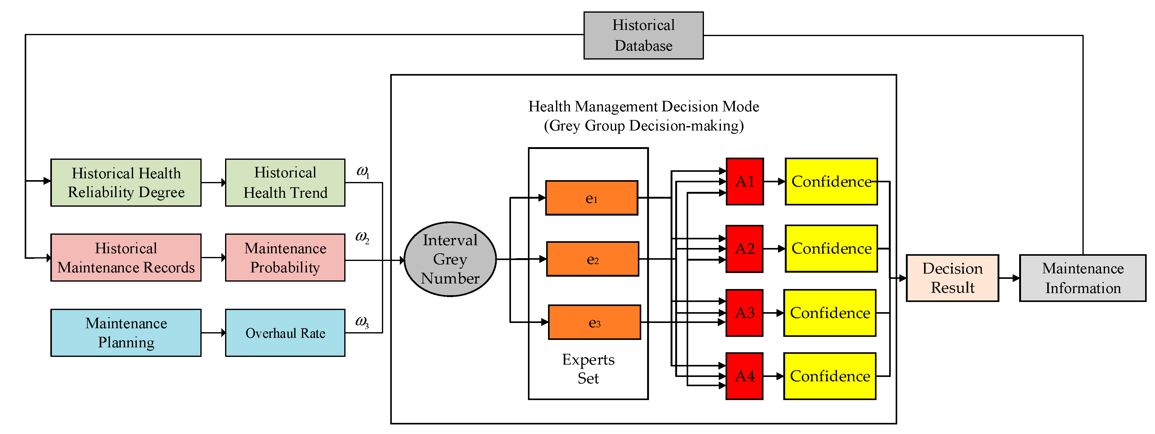
2.3. Grey Group Decision-Making
2.3.1. Grey Risk Decision-Making
2.3.2. Grey Group Decision Model for Decision-Making
2.4. The Process of Health Management Decision Method Based on Grey Group Decision
3. Experimental Setup and Analytical Discussion
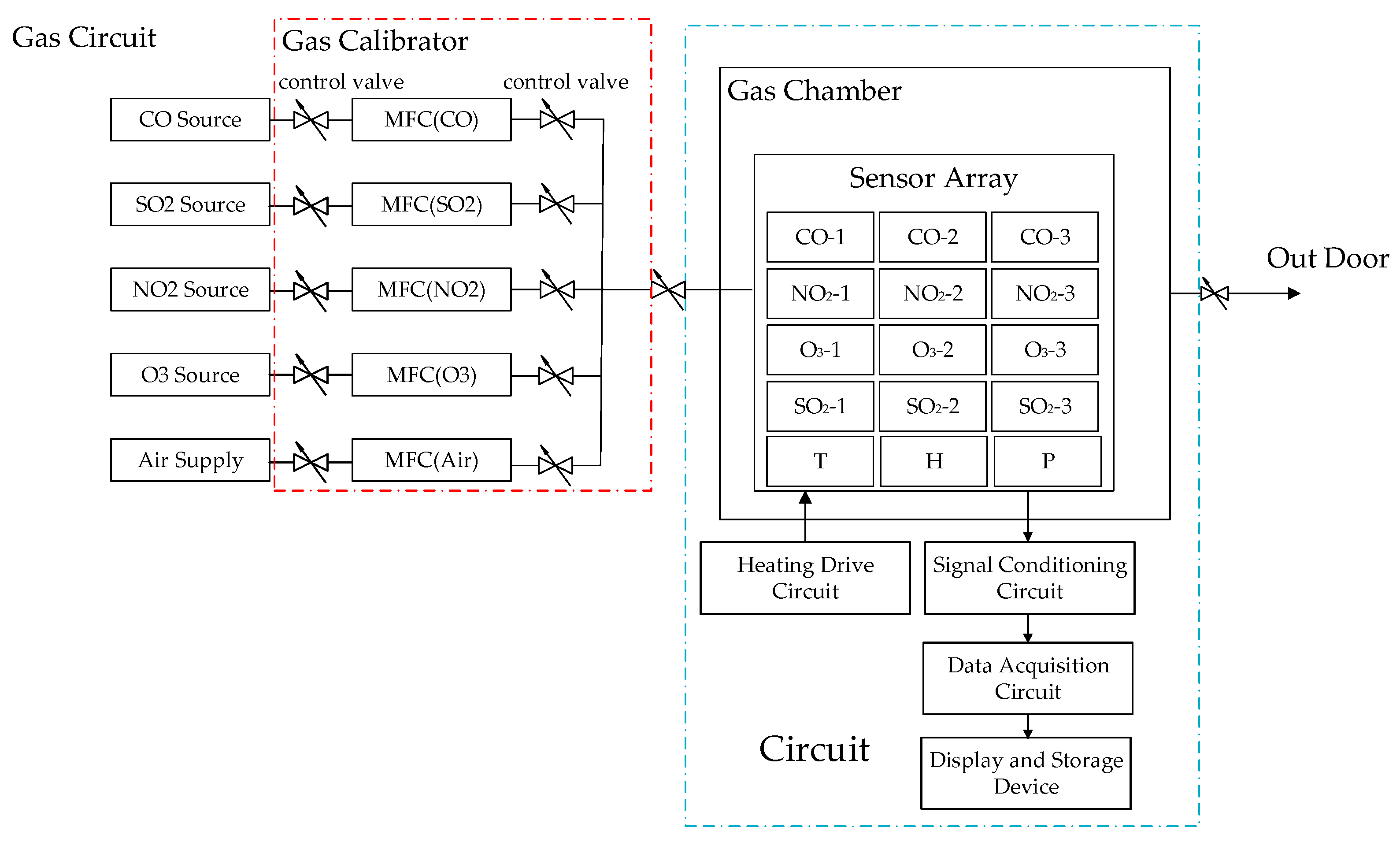
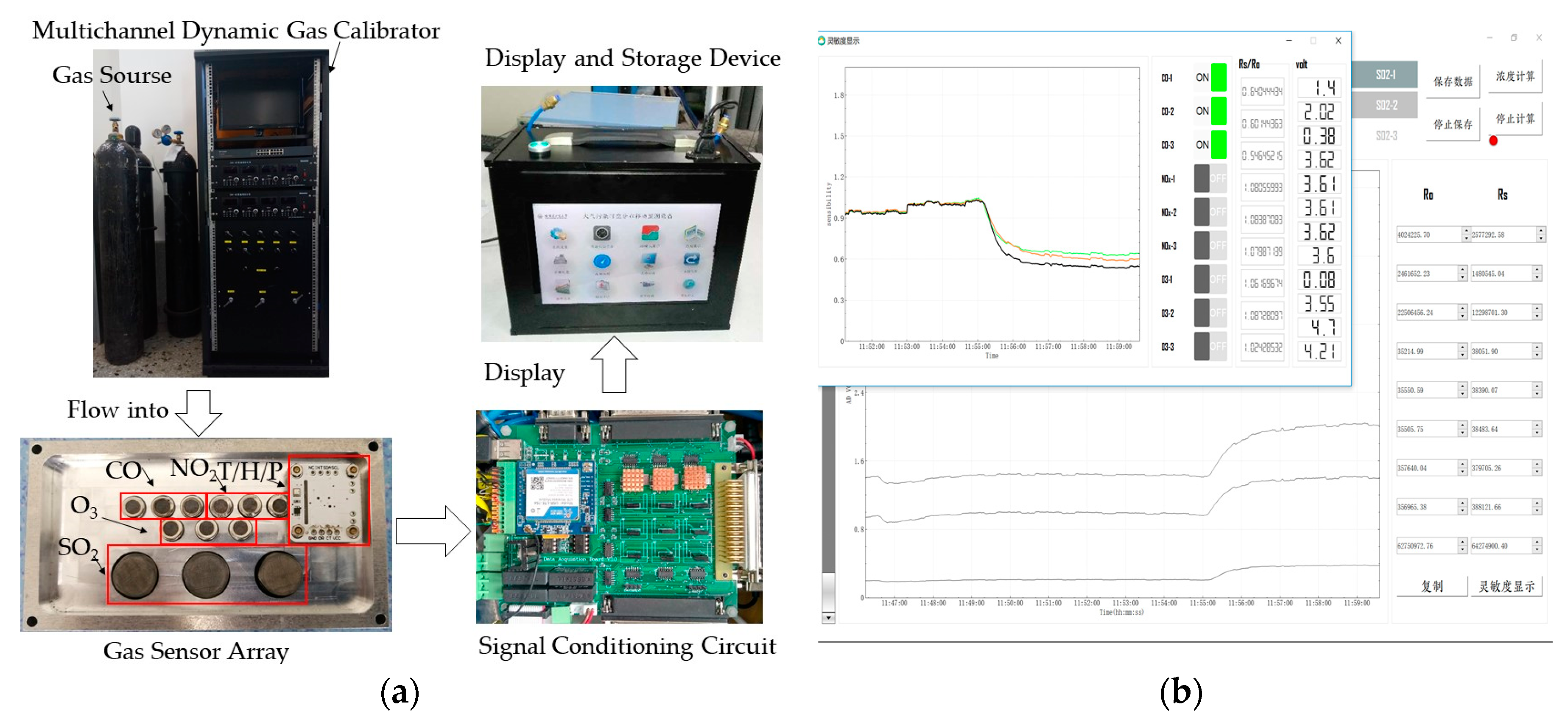
3.1. Sensor System Experimental System
3.2. Experiment Data
4. Results and Analysis
5. Conclusions
Author Contributions
Funding
Acknowledgments
Conflicts of Interest
References
- Fonollosa, J.; Vergara, A.; Huerta, R. Algorithmic mitigation of sensor failure: Is sensor replacement really necessary? Sens. Actuators B Chem. 2013, 183, 211–221. [Google Scholar] [CrossRef]
- Korotcenkov, G.; Cho, B. Engineering approaches for the improvement of conductometric gas sensor parameters: Part 1. Improvement of sensor sensitivity and selectivity (short survey). Sens. Actuators B Chem. 2013, 188, 709–728. [Google Scholar] [CrossRef]
- Korotcenkov, G.; Cho, B. Engineering approaches to improvement of conductometric gas sensor parameters. Part 2: Decrease of dissipated. (consumable) power and improvement stability and reliability. Sens. Actuators B Chem. 2014, 198, 316–341. [Google Scholar] [CrossRef]
- Fernandez, L.; Gutierrez-Galvez, A.; Marco, S. Robustness to Sensor Damage of a Highly Redundant Gas Sensor Array. Procedia Eng. 2014, 87, 851–854. [Google Scholar]
- Romain, A.C.; André, P.; Nicolas, J. Three years experiment with the same tin oxide sensor arrays for the identification of malodorous sources in the environment. Sens. Actuators B Chem. 2002, 84, 271–277. [Google Scholar] [CrossRef]
- Romain, A.C.; Nicolas, J. Long term stability of metal oxide-based gas sensors for e-nose environmental applications: An overview. Sens. Actuators B Chem. 2009, 146, 502–506. [Google Scholar] [CrossRef]
- Lazarescu, M.T. Design and Field Test of a WSN Platform Prototype for Long-Term Environmental Monitoring. Sensors 2015, 15, 9481–9518. [Google Scholar] [CrossRef] [PubMed]
- Chen, Y.; Bouferguene, A.; Al-Hussein, M. Analytic Hierarchy Process-Simulation Framework for Lighting Maintenance Decision-Making Based on the Clustered Network. J. Perform. Constr. Facil. 2018, 32, 04017114. [Google Scholar] [CrossRef]
- Dababneh, F.; Li, L.; Shah, R.; Haefke, C. Demand Response Driven Production and Maintenance Decision Making for Cost Effective Manufacturing. J. Manuf. Sci. Eng. 2018, 140, 061008. [Google Scholar] [CrossRef]
- Chen, D.; Trivedi, K.S. Optimization for condition-based maintenance with semi-Markov decision process. Reliab. Eng. Syst. Saf. 2017, 90, 25–29. [Google Scholar] [CrossRef]
- Tsui, K.L.; Chen, N.; Zhou, Q.; Hai, Y.; Wang, W. Prognostics and health management: A review on data driven approaches. Math. Probl. Eng. 2015, 6, 1–17. [Google Scholar] [CrossRef]
- Bai, G.; Wang, P.; Hu, C. A self-cognizant dynamic system approach for prognostics and health management. J. Power Sources 2015, 278, 163–174. [Google Scholar] [CrossRef]
- Coble, J.; Ramuhalli, P.; Bond, L.; Hines, J.W.; Upadhyaya, B. A review of prognostics and health management applications in nuclear power plants. Int. J. Progn. Health Manag. 2015, 6, 1–22. [Google Scholar]
- Shen, Z.; He, Z.; Chen, X.; Sun, C.; Liu, Z. A Monotonic Degradation Assessment Index of Rolling Bearings Using Fuzzy Support Vector Data Description and Running Time. Sensors 2012, 12, 10109–10135. [Google Scholar] [CrossRef] [PubMed]
- Sohaib, M.; Kim, C.H.; Kim, J.M. A Hybrid Feature Model and Deep-Learning-Based Bearing Fault Diagnosis. Sensors 2017, 17, 2876. [Google Scholar] [CrossRef] [PubMed]
- Wang, J.; Wang, X.; Wang, L. Modeling of BN Lifetime Prediction of a System Based on Integrated Multi-Level Information. Sensors 2017, 17, 2123. [Google Scholar] [CrossRef] [PubMed]
- Agarwal, V.; Lybeck, N.J.; Bickford, R.; Rusaw, R. Development Of Asset Fault Signatures For Prognostic And Health Management in the Nuclear Industry; Prognostics and Health Management: Austin, TX, USA, 2015; pp. 1–7. [Google Scholar]
- Kumar, S.; Pecht, M. Modeling approaches for prognostics and health management of electronics. Int. J. Perform. Eng. 2010, 6, 222–229. [Google Scholar]
- Carnero, M.C.; Gómez, A. A multicriteria decision making approach applied to improving maintenance policies in healthcare organizations. Bmc Me. Inf. Decis. Mak. 2016, 16, 47. [Google Scholar] [CrossRef] [PubMed]
- Alaswad, S.; Xiang, Y. A review on condition-based maintenance optimization models for stochastically deteriorating system. Reliab. Eng. Syst. Saf. 2017, 157, 54–63. [Google Scholar] [CrossRef]
- Shen, Z.; Wang, Q. Failure detection, isolation, and recovery of multifunctional self-validating sensor. IEEE Trans. Instrum. Meas. 2012, 61, 3351–3362. [Google Scholar] [CrossRef]
- Chen, Y.; Xu, Y.; Yang, J. Fault detection, isolation, and diagnosis of status self-validating gas sensor arrays. Rev. Sci. Instrum. 2016, 87, 045001. [Google Scholar] [CrossRef] [PubMed]
- Chen, Y.; Jiang, S.; Yang, J.; Song, K.; Wang, Q. Grey bootstrap method for data validation and dynamic uncertainty estimation of self-validating multifunctional sensors. Chemometr. Intell. Lab. Syst. 2015, 146, 63–76. [Google Scholar] [CrossRef]
- Song, K.; Wang, Q.; Li, J.; Zhang, H. In quantitative measurement of gas component using multisensor array and NPSO-based LS-SVR. Instrum. Meas. Technol. Conf. 2013, 80, 1740–1743. [Google Scholar]
- Shen, Z.; Wang, Q.; Zhu, F. Data-driven health evaluation of multifunctional self-validating sensor using health reliability degree. Inf. Technol. J. 2012, 11, 1597–1604. [Google Scholar] [CrossRef]
- Shen, Z.; Wang, Q. A Novel Health Evaluation Strategy for Multifunctional Self-Validating Sensors. Sensors 2013, 13, 587–610. [Google Scholar] [CrossRef] [PubMed]
- Feng, Z.G.; Wang, Q. Research on health evaluation system of liquid-propellant rocket engine ground-testing bed based on fuzzy theory. Acta Astronaut. 2007, 61, 840–853. [Google Scholar] [CrossRef]
- Xia, T.; Xi, L.; Zhou, X.; Lee, J. Dynamic maintenance decision-making for series–parallel manufacturing system based on MAM–MTW methodology. Eur. J. Oper. Res. 2012, 221, 231–240. [Google Scholar] [CrossRef]
- Berges, L.; Galar; Gustafson, A.; Tormos, B. Maintenance decision making based on different types of data fusion. Eksploat. i Niezawodn.-Maint. Reliab. 2012, 14, 135–144. [Google Scholar]
- Cates, G.L.; Skinner, C.H.; Watson, T.S.; Meadows, T.J.; Weaver, A.; Jackson, B. Instructional effectiveness and instructional efficiency as considerations for data-based decision making: An evaluation of interspersing procedures. Sch. Psychol. Rev. 2003, 32, 601–616. [Google Scholar]
- Aughenbaugh, J.M.; Herrmann, J.W. Reliability-based decision making: A comparison of statistical approaches. J. Stat. Theory Pract. 2009, 3, 289–303. [Google Scholar] [CrossRef][Green Version]
- Liu, W.B.; Wang, Q.F.; Gao, J.J.; Zhong, X.; Liang, G.H. Reliability-centered intelligent maintenance decision-making model. J. Beijing Univ. Technol. 2012, 38, 672–677. [Google Scholar]
- Wang, A.; Jiang, J.; Zhang, H. Multi-sensor Image Decision Level Fusion Detection Algorithm Based on D-S Evidence Theory. In Proceedings of the Fourth International Conference on Instrumentation and Measurement, Computer, Communication and Control, Harbin, China, 18–20 September 2014; pp. 620–623. [Google Scholar]
- He, Z.; Zhang, H.; Zhao, J.; Qian, Q. Classification of power quality disturbances using quantum neural network and DS evidence fusion. Eur. Trans. Electr. Power 2013, 22, 533–547. [Google Scholar] [CrossRef]
- Wang, H.; Lin, D.; Qiu, J.; Du, Z.; He, B. Research on Multiobjective Group Decision-Making in Condition-Based Maintenance for Transmission and Transformation Equipment Based on D-S Evidence Theory. IEEE Trans. Smart Grid 2015, 6, 1035–1045. [Google Scholar] [CrossRef]
- Lin, S.; Li, C.; Xu, F.; Li, W. The strategy research on electrical equipment condition-based maintenance based on cloud model and grey D-S evidence theory. Intell. Decis. Technol. 2018, 3, 1–10. [Google Scholar] [CrossRef]
- Mehta, P.; Werner, A.; Mears, L. Condition based maintenance-systems integration and intelligence using Bayesian classification and sensor fusion. J. Intell. Manuf. 2015, 26, 331–346. [Google Scholar] [CrossRef]
- Herrle, S.R.; Corbett Jr, E.C.; Fagan, M.J.; Moore, C.G.; Elnicki, D.M. Bayes’ theorem and the physical examination: Probability assessment and diagnostic decision making. Acad. Med. J. Assoc. Am. Med. Coll. 2011, 86, 618. [Google Scholar] [CrossRef] [PubMed]
- Lin, P.C.; Gu, J.C.; Yang, M.T. Intelligent maintenance model for condition assessment of circuit breakers using fuzzy set theory and evidential reasoning. IET Gener. Transm. Distrib. 2014, 8, 1244–1253. [Google Scholar] [CrossRef]
- Yin, K.; Yang, B.; Li, X. Multiple Attribute Group Decision-Making Methods Based on Trapezoidal Fuzzy Two-Dimensional Linguistic Partitioned Bonferroni Mean Aggregation Operators. Int. J. Environ. Res. Public Health 2018, 15, 194. [Google Scholar] [CrossRef] [PubMed]
- Chen, S.; Cheng, S.; Chiou, C. Fuzzy multiattribute group decision making based on intuitionistic fuzzy sets and evidential reasoning methodology. Inf. Fusion 2016, 27, 215–227. [Google Scholar] [CrossRef]
- Efe, B. An integrated fuzzy multi criteria group decision making approach for ERP system selection. Appl. Soft Comput. 2016, 38, 106–117. [Google Scholar] [CrossRef]
- Joshi, D.; Kumar, S. Interval-valued intuitionistic hesitant fuzzy Choquet integral based TOPSIS method for multi-criteria group decision making. Eur. J. Oper. Res. 2016, 248, 183–191. [Google Scholar] [CrossRef]
- Pramanik, S.; Pramanik, S.; Giri, B.C. TOPSIS method for multi-attribute group decision-making under single-valued neutrosophic environment. Neural Comput. Appl. 2016, 27, 727–737. [Google Scholar]
- Wang, H.; Lin, D.; Qiu, J.; Ao, L.; Du, Z.; He, B. Research on multiobjective group decision-making in condition-based maintenance for transmission and transformation equipment based on D-S evidence theory. IEEE Trans. Smart Grid 2015, 6, 1035–1045. [Google Scholar] [CrossRef]
- Peng, J.; Wang, J.; Wang, J.; Zhang, H.; Chen, X. Simplified neutrosophic sets and their applications in multi-criteria group decision-making problems. Int. J. Comput. Intell. Syst. 2016, 47, 2342–2358. [Google Scholar] [CrossRef]
- Liu, P.; Chen, S.M. Multiattribute group decision making based on intuitionistic 2-tuple linguistic information. Inf. Sci. 2018, 430, 599–619. [Google Scholar] [CrossRef]
- Manzardo, A.; Ren, J.; Mazzi, A.; Scipioni, A. A grey-based group decision-making methodology for the selection of hydrogen technologies in life cycle sustainability perspective. Int. J. Hydrog. Energy 2012, 37, 17663–17670. [Google Scholar] [CrossRef]
- Liu, P.; Chu, Y.; Li, Y. The multi-attribute group decision-making method based on the interval grey uncertain linguistic generalized hybrid averaging operator. Neural Comput. Appl. 2015, 26, 1395–1405. [Google Scholar] [CrossRef]


| Solution Set | Health Status Level | Health Description | Maintenance Level |
|---|---|---|---|
| A1 | Health (HS) | healthy condition | No maintenance |
| A2 | Subhealth (SHS) | normal range | Preventive maintenance |
| A3 | failure edge (FES) | fault edge | Corrective maintenance |
| A4 | Failure (FS) | fault condition | Immediate maintenance |
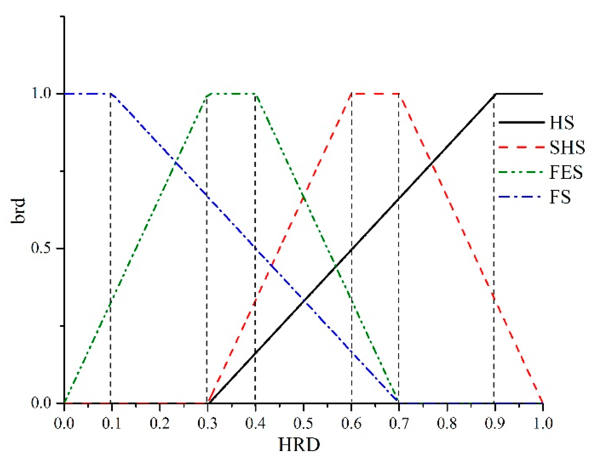
| Solution Set | Range of Health Reliability Degree | Health Status Level |
|---|---|---|
| A1 | 0.9 ≤ HRD ≤ 1 | Healthy |
| A2 | 0.6 ≤ HRD < 0.9 | Subhealthy |
| A3 | 0.2 ≤ HRD < 0.6 | Failure edge |
| A4 | 0 ≤ HRD < 0.2 | Failure |
| HRD Based on Grey Theory |
|---|
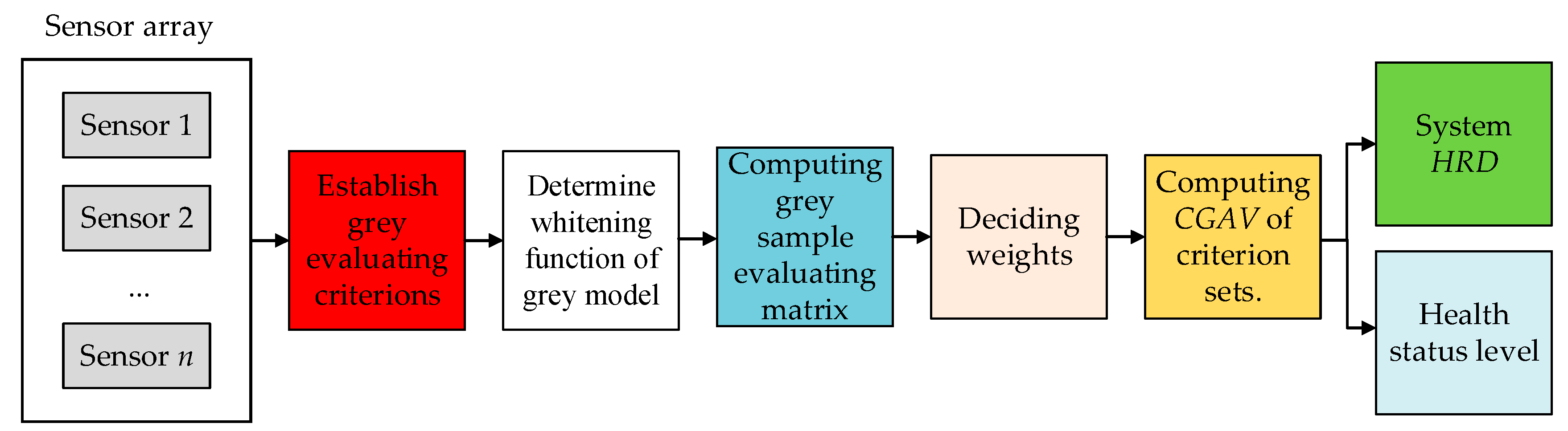
| Input: Output of the sensor system Output: Health Reliability Degree Procedure: Step 1: Establish the grey evaluating criterions, which is shown as (HS, SHS, FES, FS). Step 2: Determine the whitening function of the grey model according to Equations (1)–(4). Step 3: Compute decision weights by using information entropy method. Step 4: Compute Grey Sample Evaluating (GSE) Matrix by (5). Step 5: Calculate the CGAV under evaluating criterion sets. Step 6: Calculate HRD by RVM. |
| Grey Group Decision-Making Algorithm |
|---|
| Input: Historical Health Reliability Degree (HHRD): The parameter is composed of the last n HRDs. Maintenance Probability (MP): Maintenance probability is equal to history maintenance times/total test times. Overhaul Rate (OR): Overhaul rate is equal to the next inspection time/overhaul cycle. Output: Decision Result: The parameter is the level of the maintenance decision-making. The size of the framework is four: {no maintenance, preventive maintenance, corrective maintenance, immediate maintenance} Confidence: The parameter is output vector of the maintenance decision-making confidence. Procedure: Step 1: Calculate the interval grey numbers of each decision result for each evidence in the decision framework under each decision method. The interval grey number is expressed as , . represents the grey number lower limit and is the grey number upper limit (i = 1, 2, 3, 4, j = 1, 2, 3, s = 1, 2, 3). Step 2: According to the upper-lower limit in the interval grey number in Step 1, establish the comprehensive decision matrix (CDM) of each decision method as shown in Table 5. Step 3: By utilizing the interval grey number weakening transformation, the decision matrix of three decision methods is initialized and transformed to obtain the standardized decision matrix. Step 4: Calculate the weight of each decision method. First, determine the effect vector of the three decision methods for all decision frameworks according to the standardized decision matrix in Step 3. The matrix elements are the effect vectors of the three decision methods for each decision result in the decision framework. Then, according to the interval grey number vector distance formula and the weight of each evidence attribute ωj(j = 1, 2, 3), the space projector distance of each effect vector is calculated. Finally, the ratio between the vector distance of a decision method and the sum of effect vector distance for the other decision methods is the weight coefficient λs(s = 1, 2, 3, 4) of the decision method. Step 5: Calculate the comprehensive decision results. According to the maintenance decision result of the experts, the confidence of each decision result corresponding to the four decision frames can be obtained. Finally, according to the weight coefficients of each decision method that were obtained in Step 4, the final decision result is obtained by applying weighted averaging to the confidence. |
| Health Status Level |
|---|
| Step 1: to calculate the health level of the decision framework and the confidence of every evidence. Step 2: In grey group decision, the weight vector of each evidence attribute is ω = (ω1, ω2, ω3) Step 3: calculate the decision confidence for the expert set by . Step 4: the weight vector for each experts ωe = (ωe1, ωe2, ωe3) is obtained by entropy weight method. Step 5: calculate the confidence of the final health status level by . |
| Failure | Name | Failure Feature and Form | Failure Place | Failure Prevention and Control Measures |
|---|---|---|---|---|
| F1 | Sensor disconnect | Step Response. Lower than lower threshold | Target gas sensor | Check the sensor pin, change the target sensor |
| F2 | Sensor overload | Step Response. Above upper threshold | Target gas sensor | Check the sensor pin, change the target sensor |
| F3 | Sensor poisoned | No response or irregular fluctuation | Target gas sensor | Change the target sensor |
| F4 | Sensor drift | Slowly varying. Baseline offset | Target gas sensor | Increase the preheating time, change the target sensor |
| F5 | Abnormal changed | Output fluctuation | Target gas sensor | Check and replace the filter capacitor, check and replace the power supply module, change the target sensor |
| F6 | Heater circuit failure | Sensor has no response. Heater has no input. | Target gas sensor circuit | Circuit connection check, change the chips |
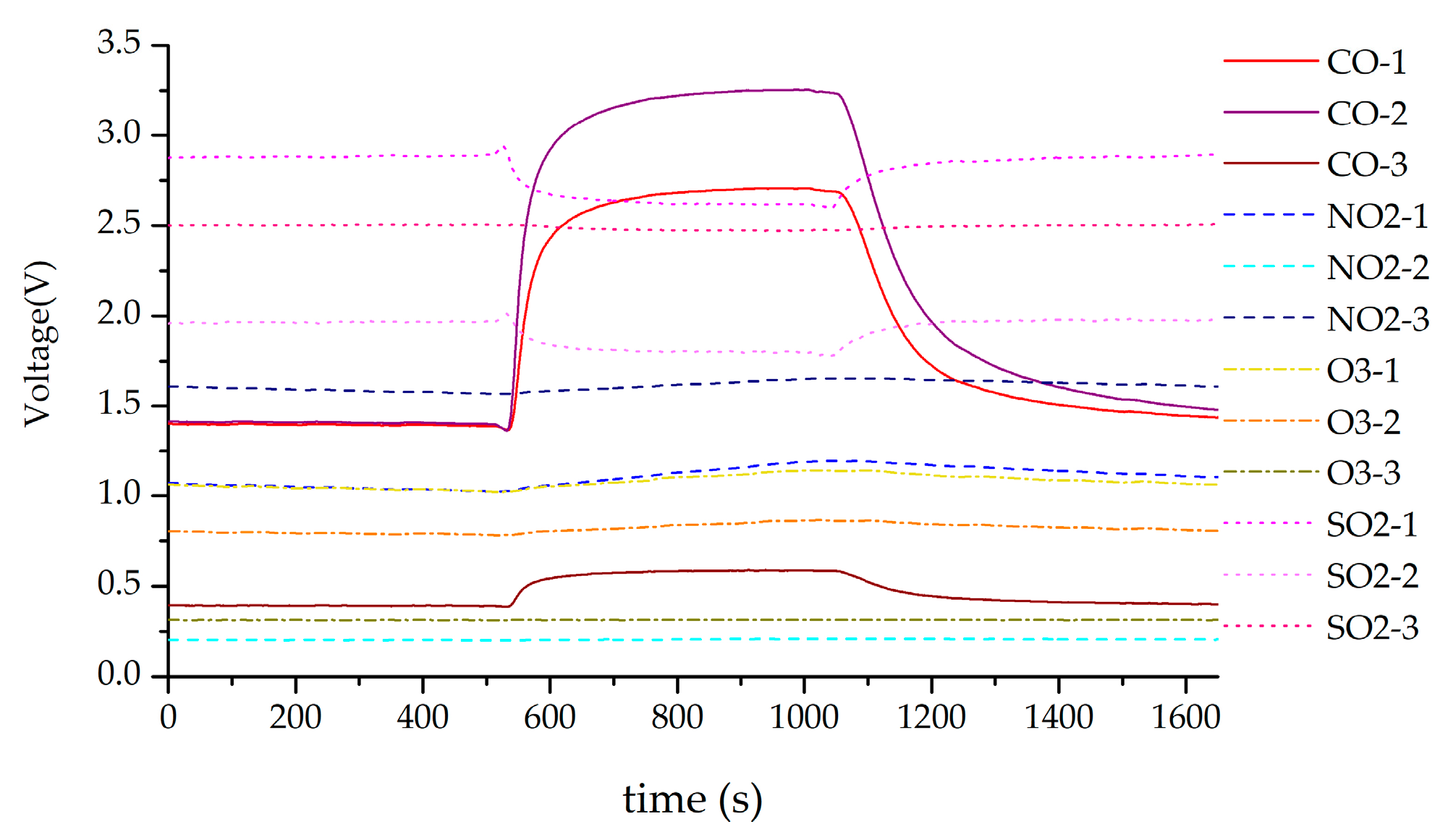
| Sensor | Range | Unit | Sensor | Range | Unit |
|---|---|---|---|---|---|
| CO-1 | 1–4 | V | O3-1 | 0.15–1.8 | V |
| CO-2 | 1–4 | V | O3-2 | 0.15–0.9 | V |
| CO-3 | 0.3–1.8 | V | O3-3 | 0.15–0.4 | V |
| NO2-1 | 0.3–5 | V | SO2-1 | 2–5 | V |
| NO2-2 | 0.3–5 | V | SO2-2 | 1.3–5 | V |
| NO2-3 | 0.1–1.5 | V | SO2-3 | 1.3–3.7 | V |
| T | 15–50 | °C | H | 20–65 | %RH |
| P | 0.09–0.12 | Kpa |
| Evidence | A1 | A2 | A3 | A4 |
|---|---|---|---|---|
| 1 | 0.8150 | 0.3930 | 0.0039 | 0 |
| 2 | 0.8648 | 0.3357 | 0.0029 | 0 |
| 3 | 0.8568 | 0.3447 | 0.0029 | 0 |
| 4 | 0.8556 | 0.3457 | 0.0031 | 0 |
| 5 | 0.7337 | 0.4792 | 0.0057 | 0 |
| 6 | 0.9388 | 0.2373 | 0.0014 | 0 |
| 7 | 0.9393 | 0.2449 | 0.0014 | 0 |
| u1 | u2 | u3 | ||||
|---|---|---|---|---|---|---|
| Grey Interval | Whitening Degree | Grey Interval | Whitening Degree | Grey Interval | Whitening Degree | |
| A1 | [0.8562, 0.8617] | 0.8589 | [0.8690, 0.8707] | 0.8698 | [1, 1] | 1 |
| A2 | [0.1383, 0.1438] | 0.1411 | [0.5853, 0.5920] | 0.5937 | [0.1650, 0.1683] | 0.1667 |
| A3 | [0, 0] | 0 | [0, 0] | 0 | [0, 0] | 0 |
| A4 | [0, 0] | 0 | [0, 0] | 0 | [0, 0] | 0 |
| weight | 0.7719 | 0.05 | 0.1781 | |||
| u1 | u2 | u3 | ||||
|---|---|---|---|---|---|---|
| Grey Interval | Whitening Degree | Grey Interval | Whitening Degree | Grey Interval | Whitening Degree | |
| A1 | [0.8860, 0.9026] | 0.8943 | [0.8690, 0.8707] | 0.8698 | [1, 1] | 1 |
| A2 | [0.0974, 0.1140] | 0.1057 | [0.5853, 0.5920] | 0.5937 | [0.1650, 0.1683] | 0.1667 |
| A3 | [0, 0] | 0 | [0, 0] | 0 | [0, 0] | 0 |
| A4 | [0, 0] | 0 | [0, 0] | 0 | [0, 0] | 0 |
| weight | 0.7719 | 0.05 | 0.1781 | |||
| u1 | u2 | u3 | ||||
|---|---|---|---|---|---|---|
| Grey Interval | Whitening Degree | Grey Interval | Whitening Degree | Grey Interval | Whitening Degree | |
| A1 | [0.6579, 0.6611] | 0.6595 | [0.8690, 0.8707] | 0.8698 | [1, 1] | 1 |
| A2 | [0.3348, 0.3381] | 0.3364 | [0.5853, 0.5920] | 0.5937 | [0.1650, 0.1683] | 0.1667 |
| A3 | [0.0040, 0.0041] | 0.0040 | [0, 0] | 0 | [0, 0] | 0 |
| A4 | [0, 0] | 0 | [0, 0] | 0 | [0, 0] | 0 |
| weight | 0.7719 | 0.05 | 0.1781 | |||
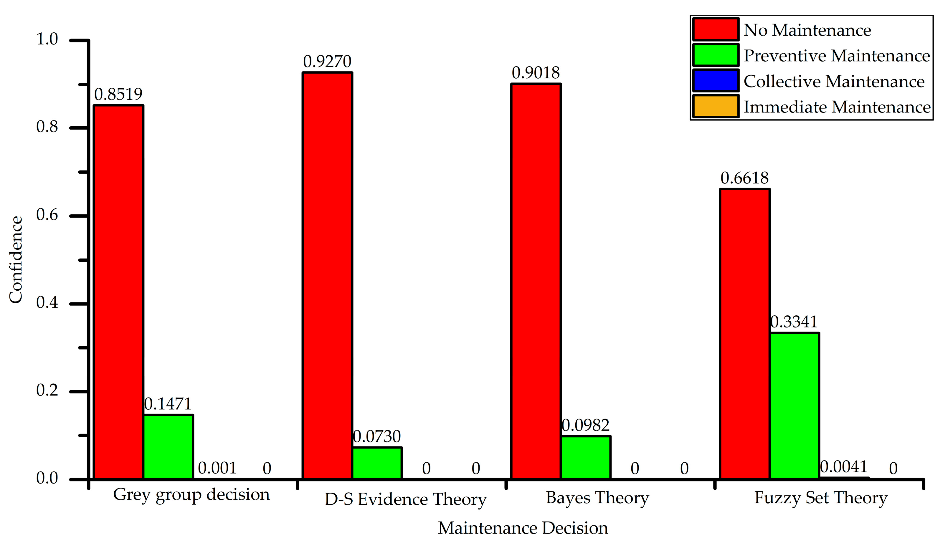
| Method | Rank | Maintenance Suggestion |
|---|---|---|
| Grey Group Decision | A1 > A2 > A3 > A4 | A1: No Maintenance |
| D-S evidence Theory | A1 > A2 > A3 > A4 | A1: No Maintenance |
| Bayes Theory | A1 > A2 > A3 > A4 | A1: No Maintenance |
| Fuzzy Set Theory | A1 > A2 > A3 > A4 | A1: No Maintenance |
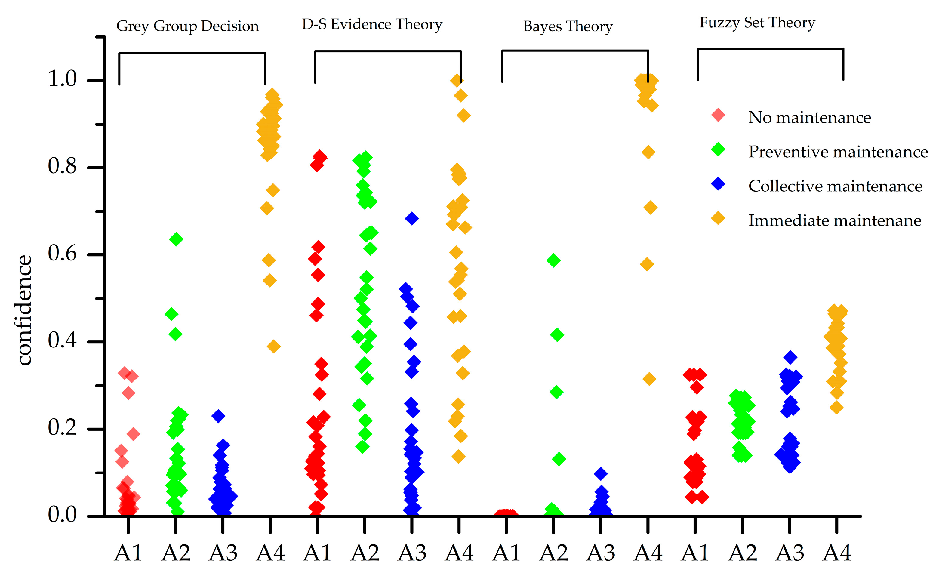
| Health Status Level | Grey Group Decision | D-S Evidence Theory | Bayes Theory | Fuzzy Set Theory |
|---|---|---|---|---|
| A1 | 100% | 100% | 94% | 100% |
| A2 | 100% | 93% | 100% | 94% |
| A3 | 95% | 40% | 95% | 60% |
| A4 | 98% | 49% | 98% | 93% |
| average | 98.25% | 65.5% | 96.75% | 85.75% |
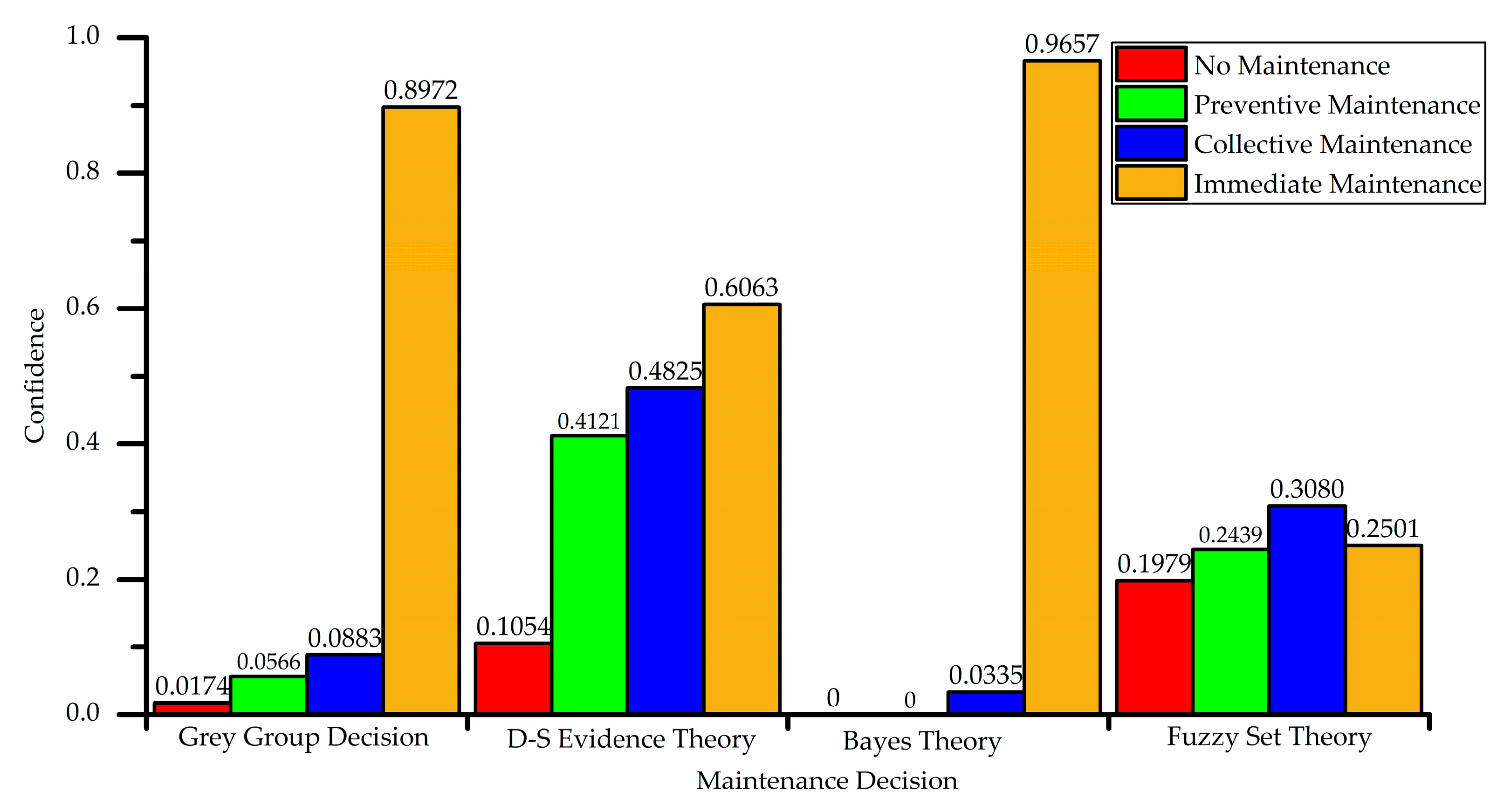
| Method | Rank | Maintenance Suggestion |
|---|---|---|
| Grey Group Decision | A4 > A3 > A2 > A1 | A4: Immediate Maintenance |
| D-S evidence Theory | A4 > A3 > A2 > A1 | A4: Immediate Maintenance |
| Bayes Theory | A4 > A3 > A2 = A1 | A4: Immediate Maintenance |
| Fuzzy Set Theory | A3 > A4 > A2 > A1 | A3: Collective Maintenance |
© 2018 by the authors. Licensee MDPI, Basel, Switzerland. This article is an open access article distributed under the terms and conditions of the Creative Commons Attribution (CC BY) license (http://creativecommons.org/licenses/by/4.0/).
Share and Cite
Song, K.; Xu, P.; Wei, G.; Chen, Y.; Wang, Q. Health Management Decision of Sensor System Based on Health Reliability Degree and Grey Group Decision-Making. Sensors 2018, 18, 2316. https://doi.org/10.3390/s18072316
Song K, Xu P, Wei G, Chen Y, Wang Q. Health Management Decision of Sensor System Based on Health Reliability Degree and Grey Group Decision-Making. Sensors. 2018; 18(7):2316. https://doi.org/10.3390/s18072316
Chicago/Turabian StyleSong, Kai, Peng Xu, Guo Wei, Yinsheng Chen, and Qi Wang. 2018. "Health Management Decision of Sensor System Based on Health Reliability Degree and Grey Group Decision-Making" Sensors 18, no. 7: 2316. https://doi.org/10.3390/s18072316
APA StyleSong, K., Xu, P., Wei, G., Chen, Y., & Wang, Q. (2018). Health Management Decision of Sensor System Based on Health Reliability Degree and Grey Group Decision-Making. Sensors, 18(7), 2316. https://doi.org/10.3390/s18072316