1. Introduction
With the increase of wireless communication, spectrum resources have become increasingly scarce. However, most primary users, or authorized users, do not use the spectrum resources allocated to them most of the time [
1]. For example, RFeye node [
2] is used to monitor the wireless spectrum at Queen Mary University of London, and most of the spectrum resources are found to be idle [
3]. TeleVision White Space (TVWS) in the Ultra High Frequency (UHF) band is the spectrum band not used by Digital Terrestrial Televisions (DTT), and Programme Making and Special Events (PMSE). The wireless communication network using TVWS can cover above 10 km in diameter, and it has strong penetration capabilities for buildings, mountains and forests. Cognitive radio devices working in TVWS can be used in rural areas where the communication infrastructure is imperfect to build a communication link among machines and improve residents’ access to the Internet. The communication regulator in the United Kingdom, the Office of Communications (Ofcom), announced that using TVWS does not need a communication license in December 2015 [
4]. Therefore, TVWS is one of the most promising opportunistic spectrum access resources.
TVWS can be used by secondary users to transmit their information to enhance spectrum utilization efficiency. Geo-location database is a way to discover available TVWS [
5]. However, this method requires a wired or wireless connection with the Geo-location database in advance [
6]. The dynamic changes in the wireless environment pose a huge challenge to this database-based approach. Therefore, we need to quickly and accurately detect whether primary users exist before using spectrum resources in TV band. According to the well-known Nyquist sampling theorem, alias free sampling requires the system sampling rate be higher than twice the maximum frequency of the signal. The currently available Analog-to-Digital Converters (ADC) often cannot satisfy the sampling rate requirement for wideband signals. Even with such an ADC, the cost is usually extremely high in terms of price and power consumption. Thus, it is attractive to conduct spectrum sensing based on sub-Nyquist sampling techniques.
Some parallel sub-Nyquist sampling schemes have been developed in recent years, such as the Modulated Wideband Converter (MWC) [
7] and the parallel Multi-Coset Sampling (MCS) [
8]. A Distributed Modulated Wideband Converter (DMWC) scheme is proposed, and a sensor node is considered to be an MWC channel in DMWC [
9]. DMWC combines cooperative spectrum sensing and MWC techniques for wideband spectrum sensing. A Random Triggering-based Modulated Wideband Compressive Sampling (RT-MWCS) is also designed for repetitive sparse wideband signals [
10]. However, the input signal is multiplied with the periodic Pseudo-Random Binary Sequence (PRBS) by a mixer in MWC, and it is difficult to suppress the unwanted harmonics due to the usage of PRBS instead of a single-tone as the local oscillator signal. Parallel MCS is another promising sub-Nyquist sampling scheme which has several sub-ADCs working parallelly. The sampling clocks of these sub-ADCs have the same frequency but different phases. Time-Interleaved ADC (TIADC) platform can be used to implement parallel MCS to further improve the time resolution of TIADC. Just as mismatches among sub-ADCs, mainly offset mismatch, gain mismatch and sampling clock skew, degrade the Spurious Free Dynamic Range (SFDR) of a TIADC system [
11,
12], they can also severely deteriorate spectrum-sensing performance based on parallel MCS.
The mismatch problem in parallel MCS can be avoided in single-channel sampling structure. A single-channel Non-Uniform Sampling (NUS) structure is design, in which a custom-designed Sample/Hold (S/H) and a commercial ADC are used [
13]. Then a nonlinear compressive sensing algorithm is used to reconstruct the signal. The computational complexity of reconstruction is reduced by emulating MCS in NUS [
14]. The signal sparsity is exploited to reduce the sampling rate requirement in [
7,
8,
13,
14], and the Nyquist sampling rate is required when the signal is not sparse.
The above mentioned sub-Nyquist sampling methods concentrate on signal reconstruction, while one may only be interested in the power spectrum in some practical applications, such as cognitive radio and spectrum monitoring. A Single-Channel Modulated Wideband Converter (SCMWC) scheme is proposed, and experiment circuit is designed using commercial Integrated Circuits (ICs) to verify the feasibility of SCMWC [
15]. Only power spectrum information is estimated to conduct spectrum sensing in [
15]. The signal statistical property is exploited to estimate finite resolution power spectrum of signal without requiring the signal to be sparse [
16]. The mean and variance of the finite resolution power spectrum estimator are investigated when the number of sub-Nyquist samples is limited [
17]. The signal statistical property is also utilized to estimate power spectrum of signal in [
18]. After the power spectrum is obtained, the primary user is detected using the energy detection method. However, the estimation of power spectrum requires a large amount of calculation. Compared with the multi-band model [
18], authors in [
19] consider both multi-band and multi-tone models, the case of sparse and non-sparse, and known and unknown carrier frequencies. They derive minimum sampling rate requirement for each setting without noise and provide power spectrum reconstruction techniques to achieve these minimum sampling rates. The least squares method is used to estimate the signal power spectrum, and the full rank condition of the system matrix is viewed as a circular sparse ruler design problem [
20,
21].
In this paper, we propose a spectrum-sensing method based on single-channel sub-Nyquist sampling. To begin with, to avoid the mismatch problem among sub-ADCs in parallel MCS [
16,
17,
18], a serial MCS structure is proposed. The proposed serial MCS mainly consists of a S/H, an ADC and two different periodic non-uniform sampling clocks. The clocks of S/H and ADC are provided by these two different periodic non-uniform sampling clocks. The S/H functions similar to an analog signal register, which can shift the high sampling rate requirement for wideband signals from ADC to S/H. Although the sampling rate requirement for the ADC in serial MCS is higher than that in parallel MCS, there is no mismatch problem and the implementation size is smaller. Moreover, to reduce the computational complexity in [
18], we propose an efficient spectrum-sensing algorithm. The frequency-smoothing property of the power spectrum estimator is exploited to estimate the frequency-smoothed power spectrum of the signal. Since the frequency bins in a frequency-smoothing window are highly correlated, spectrum sensing only needs estimate power spectrum at partial frequency bins, which will save a large amount of computational cost. Then finally, to use the least square algorithm to estimate the power spectrum, we must ensure that the system matrix has full column rank. Whether the system matrix has full column rank is determined by the sampling pattern design, which is further proved to be a minimal circular sparse ruler design problem with an additional constraint. The sampling pattern design method in [
20,
21] is only suitable for the traditional parallel MCS. We consider the sampling pattern design for the proposed serial MCS. Simulations show that mismatches among sub-ADCs deteriorate the spectrum-sensing performance seriously, especially the false alarm probability, while the proposed MCS combined with the proposed efficient spectrum-sensing algorithm not only has outstanding spectrum-sensing performance, but also requires less computational load.
This paper is organized as follows:
Section 2 presents the signal model and forms the problem. The sampling structure and sampling process of the proposed serial MCS are described in
Section 3.
Section 4 firstly introduces a power spectrum estimation method and then proposes an efficient spectrum-sensing algorithm. The sampling pattern design of the proposed serial MCS is developed in
Section 5. Simulation results are given in
Section 6. Simulations take some practical parameters into account, such as Signal-to-Noise Ratio (SNR), compression ratio, and acquisition time.
Section 7 discusses using the spectrum-sensing module to receive communication signals.
2. Signal Model and Problem Formulation
The spectrum resource we are interested in is the UHF TV band, and its frequency range is from 470 MHz to 790 MHz. The bandwidth of a channel is 8 MHz, and there are 40 channels in total. Assume that
users are active during spectrum sensing.
users may comprise of both primary users and other secondary users. Without loss of generality, the
k-th user can be represented as:
where
is a sequence of transmitted symbol,
is the pulse-shaping function,
is the symbol duration and
is the carrier frequency.
The practical wireless transmission channel mainly has two effects on the signal, one is log-normal shadowing which is a typical large-scale fading, the other is Rayleigh fading which is a typical small-scale fading [
22,
23,
24]. To begin with, Large-scale fading denotes the average signal power attenuation caused by a wide range of movements. This kind of fading is mainly caused by the prominent terrain between the transmitter and the receiver. Experimental results show that the large-scale fading can be represented by a log-normal random variable [
23]. Thus, large-scale fading can be expressed as:
where the reference distance
is in the far field of the transmitting antenna, the reference power
is usually obtained by field test, the path loss exponent
depends on the carrier frequency, antenna height and transmission environment,
denotes a Gaussian random variable with variance
and unit dB. Thus, the received signal affected by large-scale fading can be represented as:
where
denotes the attenuation between the
-th primary user and the cognitive radio device. Moreover, the primary user may arrive at the cognitive radio device via multiple paths, which can be modeled as Rayleigh fading. In other words, the envelope of the signal subjects to the Rayleigh distribution. The probability density function of Rayleigh distribution can be expressed as:
where
denotes the amplitude of the envelop of the received signal,
denotes its average power. The
-th primary user
arrived at the cognitive radio device can be written as
where
and
denote the convolution operator and channel impulse response.
Then the signal received by the cognitive radio device is:
where
is the signal component and
is the additive white Gaussian noise.
Figure 1 shows a wideband signal with 3 active users. They occupy the 23rd, 40th and 59th channel, while the other channels are vacant. These vacant channels can be used by secondary users to transmit their information.
After the spectrum range and channel partitioning format in the UHF TV band is given, the problem of wideband spectrum sensing is to detect which channels are occupied by the primary users and which channels are vacant. A band-pass filter is firstly used to filter out the noise outside the band [470 MHz, 790 MHz], and then a mixer is utilized to demodulate the filtered signal. The demodulated signal is a band-limited signal and its bandwidth is 320 MHz. A traditional method to solve this problem is to first sample the demodulated signal at the Nyquist sampling rate, and then estimate its power spectrum. Finally, the energy detection method is used to determine whether primary users exist. The Nyquist sampling theorem states that alias-free sampling requires the sampling rate be higher than twice the maximum frequency of the signal. Therefore, the sampling rate requirement for the demodulated signal is 640 MHz, which poses a great challenge to current available ADCs. Even with such a high sampling rate ADC, it is usually unacceptable in terms of price and power consumption for some sensors and battery-powered devices. In this paper, we consider using sub-Nyquist sampling technique to conduct spectrum sensing.
3. Single-Channel Sub-Nyquist Sampling Structure
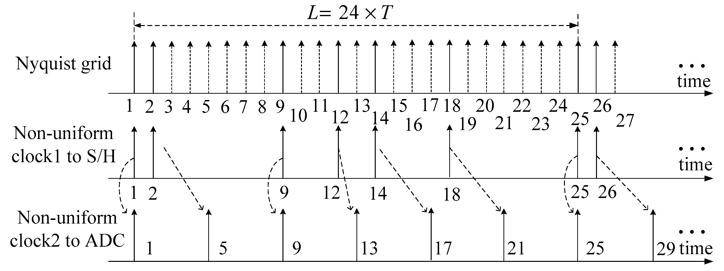
An overview of the proposed single-channel sub-Nyquist sampling scheme is shown in
Figure 2. The signal received by the antenna is first band-pass filtered to remove the out-of-band noise and interference, and then a mixer is used to demodulate the filtered signal. Finally, low-pass filter is used to remove the local oscillator signal. The demodulated signal still has a high bandwidth if we are interested in many channels. The dotted box shows the proposed serial MCS. The S/H is used to sample and temporarily store the input analog signal
. Then the subsequent ADC can sample it at a lower rate. Two periodic Pseudo-Random Binary Sequences are used as the non-uniform sampling clocks of S/H and ADC. The periodic non-uniform sampling clock provided to S/H is determined by the sampling pattern of MCS, while the periodic non-uniform sampling clock provided to ADC is dependent on not only the sampling pattern but also the sampling rate of ADC. The spectrum-sensing procedure can be summarized as follows: (1) Classifying the periodic non-uniformly sampled data into several uniform sampling sequences; (2) Power spectrum at partial frequency bins is estimated using these uniform sampling sequences; (3) Compare the estimated power spectrum with a pre-defined threshold to determine whether the primary user exists.
In detail, let
denote the signal output from the low-pass filter. Let the Nyquist sampling rate and interval of
be
and
, respectively. Let the sampling rate and interval of ADC be
and
, respectively. Let
represent the sub-Nyquist sampling factor which is defined as
.
samples are selected from
consecutive Nyquist samples in MCS. The sampling pattern
, where
is used as the sample index. Let
represent the number of samples of a coset, and the total number of periodic non-uniformly sampled data is
. We will explain in
Section 5, Sampling pattern design, that at least one pair of cosets with only
time difference should be included in the sampling pattern. The ADC cannot directly capture two samples
and
with only
time difference because the sampling interval of ADC
is greater than
. The function of S/H is to temporarily store the second coset
until the ADC has finished capturing the previous coset
.
An example of the sampling process is given in
Figure 3, where
,
,
and
. The first coset
can be sampled directly, while the second coset
must be firstly sampled by the S/H and subsequently captured by the following ADC on the fifth Nyquist time grid. Thus, the third coset
must be greater than or equal to 5, otherwise, it will lose the last coset
. The cooperation between the first and the second periodic non-uniform sampling clock ensures that two adjacent cosets with only
time difference can be captured by an ADC with sampling rate
which is much lower than
, and this is the essence of the proposed serial MCS.
The periodic non-uniformly sampled data are classified into several uniform sampling sequences. Let
represent the periodic non-uniformly sampled data output from the ADC and it can be written as:
where
is the sample obtained from the
k-th Nyquist sample block with length
L using sample index
. Please note that the number of
equals to the total number of periodic non-uniformly sampled data
. Then periodic non-uniformly sampled data
is classified into
uniform sampling sequences
Let
represent the
i-th uniform sampling sequence which corresponds to the
i-th coset
. The sampling rate and time offset of
are
and
, respectively.
uniform sampling sequences can be written in matrix form concisely:
The parameter of current available ICs should be considered in practical implementation. The sampling rate requirement for S/H is high, but the sampling rate requirement for the following ADC is low. The high sampling rate burden for wideband signals is shifted from ADC to S/H. The sampling rate and input bandwidth of current state-of-the-art S/H are 4GSPS (Giga-Samples Per Second) and 18 GHz, respectively (HMC760LC4B, Analog Devices, Inc., Norwood, MA, USA). Moreover, the jitter of the periodic non-uniform sampling clock is also an important parameter in serial MCS. The alternating rate and jitter of current state-of-the-art PRBS generator are 80 GHz and 600 fs (femtosecond), respectively [
25]. Periodic non-uniform sampling clock can also be generated using commercial parallel-to-serial converter. The alternating rate and typical jitter of current state-of-art parallel-to-serial converter are 3.2 GHz and 200 fs, respectively (MC100EP446, ON Semiconductor, Inc., Phoenix, AZ, USA).
4. Spectrum Sensing
After
uniform sampling sequences are obtained using the proposed serial MCS, they are further processed to conduct spectrum sensing. We firstly introduce a power spectrum estimation method [
18], and then an efficient spectrum-sensing algorithm is proposed.
4.1. Power Spectrum Estimation
This section mainly consists of two parts:
- (a)
Establish the theoretical model for power spectrum estimation.
- (b)
Develop an implementation method for the theoretical model.
(a). Establish the Theoretical Model for Power Spectrum Estimation
Let
denote the Fourier Transform of the demodulated signal
in
Figure 2. We first analyze the relationship between the spectrum of the
i-th uniform sampling sequence
and the original spectrum
. Define
as the Discrete Time Fourier Transform (DTFT) of the
i-th uniform sampling sequence
, and it can be written as:
where
and
is assumed to be even. The band-limited property
,
is used in the derivation from the first step to the second step. The relationship between the spectrum of the delayed signal
and the original spectrum
,
, is used in the derivation from the second step to the third step. The term
in Equation (10) can be moved to the left of the equation, and define
Equation (10) can be rewritten as
At this point, we have established the relationship between the spectrum of the
i-th uniform sampling sequence
and the original spectrum
in Equation (12) for single uniform sampling sequence
.
uniform sampling sequences, or the entire MCS system, can be expressed in matrix form concisely
where
,
,
,
and
.
The demodulated signal
comprises of signal component
and noise component
. Let
and
denote the Fourier Transform of
and
, respectively. Define
vector
and
vector
. Let
denote the covariance matrix of
, and it can be written as:
Similarly, the covariance matrix of
,
and
can be expressed as
,
and
. Equation (14) can be further written as:
The following explanation shows that the covariance matrix
is a diagonal matrix. The (
i,
j)-th element of
can be expressed as:
where the signal component
and noise component
are assumed to be independent, different primary users are assumed to be independent, and the property of stationary process is used in these derivations. The first term
in Equation (16) corresponds to a diagonal matrix with only
non-zero elements, while the second term
in Equation (16) also corresponds to a diagonal matrix but with
non-zero elements. Therefore, the covariance matrix
is a diagonal matrix with only
non-zero diagonal elements. This characteristic is used to further develop the power spectrum estimation method.
Let
and
represent the matrix vectorization operator and Kronecker product, respectively. Define
, Equation (15) can be rewritten as:
where the matrix identity
is used. The vector form of the diagonal matrix
can be further written as
, where
is the
i-th diagonal element and
is selected from the
i-th row of a
identity matrix. Further define
and a
selection matrix
which has 1 at the
j-th column and the
-th row. The vector form of the diagonal matrix
can be written as
. Equation (17) can be further expressed as
where
is a
matrix. If
has full column rank and Equation (18) is an over-determined system, then least square algorithm can be used to estimate the power spectrum
where
is the Moore-Penrose inverse of
.
(b). Develop an Implementation Method for the Theoretical Model
The theoretical model of power spectrum estimation is established in the previous section. However, the Fourier transform involved in the theoretical model is implemented through Fast Fourier Transform (FFT) in practice. In this section, the implementation method of the theoretical model in the digital domain is discussed. The main contents include: (1) Compensate the fractional delay of the uniform sampling sequences in MCS. (2) Estimate the cross-power spectrum of the uniform sampling sequences using the frequency-smoothed cyclic cross-periodogram. (3) Detect the presence of the primary user using the estimated power spectrum.
To begin with, let
represent the FFT of the
i-th uniform sampling sequence. Define a constant phasor corresponding to the
i-th uniform sampling sequence
. Equation (11) in the theoretical model compensates the fractional delay of the
i-th uniform sampling sequence of MCS. In practice, the implementation of fractional delay compensation in the digital domain can be represented as:
where
. Define
and its FFT
. Partition
into
,
and
. Define
and
. Equation (13) in the theoretical model can be written as
.
Next, to estimate the signal power spectrum using Equation (19), we should first obtain
. The element at the
i-th row and
j-th column of matrix
is
. That is, in order to estimate the power spectrum of signal using Equation (19), we should first calculate the cross-power spectrum of
and
at frequency bin
,
. A cross-power spectrum estimator [
26] is introduced to calculate the cross-power spectrum of
and
. Define
as the cyclic cross-spectrum of
and
, where
is the cyclic frequency. The frequency-smoothed cyclic cross-periodogram is used as a consistent estimator of
, and it can be written as
where
,
is the DTFT of
and
is the spectral window function. In practical digital implementation, FFT is used to calculate the DTFT. The frequency-smoothed cyclic cross-periodogram can be correspondingly written as
where
and
. Define
as
, and it can be estimated using
Thus, the frequency-smoothed cyclic cross-periodogram of
can be written as:
where
. Define the diagonal elements of
as
. Similar to Equation (19), we can estimate the power spectrum of signal using least square algorithm
where
.
Finally, the spectrum-sensing problem is subsequently regarded as a binary hypothesis testing problem,
The noise level
and estimate variance
are assumed to be known, which can be obtained from receiver calibration, but the power spectrum of signal
is unknown. Next, constant false alarm probability
is imposed across all frequency bins, and the detection threshold is determined as
where
is the tail distribution function of the standard normal distribution.
4.2. Efficient Spectrum-Sensing Algorithm
The traditional spectrum-sensing method [
18] first estimates the power spectrum of signal, and then uses the estimated power spectrum for primary user detection. However, the computational load of power spectrum estimation is heavy. The power spectrum estimation requires repeatedly solving Equation (25)
times. Therefore, the power spectrum estimation requires a large amount of computation when the number of samples of a coset
is large. Interestingly, note that the frequency-smoothed cyclic cross-periodogram is used to estimate
in Equation (24), and
is also a frequency-smoothed result of the original
. If the width of the spectral window function
is wide enough, the estimated power spectrum
at frequency bin
will contain the power spectrum information from the surrounding frequency bins
. In other words, the estimated power spectrum
will reflect the outline information of the original power spectrum. Since the power spectrum information is highly correlated at frequency bins in the spectral window, it is not necessary to estimate the power spectrum information at all frequency bins. Therefore, to reduce computational complexity, only power spectrum at partial frequency bins is estimated to conduct spectrum sensing. The proposed efficient spectrum-sensing algorithm exploits the frequency-smoothing property of the power spectrum estimator to reduce computational complexity, and it is summarized as Algorithm 1.
| Algorithm 1. Efficient Spectrum-Sensing Algorithm based on Power Spectrum at Partial Frequency Bins |
Initialization:
Classify the periodic non-uniformly sampled data to uniform sampling sequences , and calculate their FFT .
Step 1:
Implement fractional delay compensation in the frequency domain, , .
Step 2:
The width of the spectral window is chose to be . Compute the frequency-smoothed cross-periodogram of and at partial frequency bins .
Step 3:
Estimate the power spectrum at partial frequency bins .
Decision:
Compare with the predefined threshold , and a sequence of binary results can be obtained. Then the result can be obtained by flipping consecutive 1s with length less than to 0s. |
In the initializing stage, uniform sampling sequences can be obtained by classifying the periodic non-uniformly sampled data . Then the FFT of uniform sampling sequences are calculated and expressed as .
The first step achieves the function of compensating the fractional delay of uniform sampling sequences in the frequency domain. Compared with the traditional method which uses the fractional delay filter to compensate the fractional delay, this method has lower computational complexity. Detailed analysis of the reduction of computational complexity is beyond the scope of this paper.
In the second step, let denotes the interval of choosing partial frequency bins from all bins uniformly. The frequency-smoothed cross-periodogram of and at partial frequency bins is calculated. We assume that is an integer multiple of . Define as the minimum modulation bandwidth of primary user, and as the bandwidth of a frequency bin. The width of the spectral window function and are both chosen to be to obtain a smoothed version of the original power spectrum. Please note that the width of the spectral window function is very important to obtain the outline information of the original power spectrum.
The third step uses the least square method to estimate the power spectrum at partial frequency bins , which only needs repeatedly solving Equation (25) times. Compared with the traditional method which needs repeatedly solving Equation (25) times, the amount of calculation has been reduced by times.
Finally, the estimated power spectrum at partial frequency bins are compared with the predefined threshold . A sequence of binary results can be obtained after the comparison. The minimum modulation width of primary user and the width of the frequency bin can be exploited to further refine the binary sequence. Consecutive 1s with length less than are flipped to 0s, then channels with 1s are considered occupied by primary users.
Some applications are sensitive to the computational complexity of the spectrum-sensing module, such as sensor nodes and battery-powered devices. Compared with the traditional method which estimates the power spectrum at all frequency bins, the proposed efficient spectrum-sensing algorithm only estimates power spectrum at partial frequency bins, by exploiting the frequency-smoothing characteristics of the power spectrum estimator. It is reasonable to use the power spectrum information at partial frequency bins to determine whether the primary user exists because the estimate result in the third step of Algorithm 1 is the weighted average result of the original power spectrum in a spectral window function.
5. Sampling Pattern Design
The matrix
is assumed to have full column rank when the least square method is used to estimate the power spectrum in Equation (25). In fact, whether it has full column rank is determined by the sampling pattern of MCS. Let us explore the structure of matrix
. Let
and
, denote the
i-th row of matrix
and
, respectively.
and
can be further written as
and
, respectively. The structure of
matrix
is firstly explored and it can be written as:
where
is the
-th row vector of matrix
. The
selection matrix
can be written as:
Based on the structure of matrix
, it is not difficult to find that multiplying a
vector
with a
selection matrix
is equivalent to
, where
denotes the matrix dot product. Therefore, matrix
can be rewritten as:
Since the row vector
of matrix
can be written as
, the
-th row vector of matrix
can be further written as
Please note that , the -th row of matrix , has some special structure. It can be viewed as the -th row of the Discrete Fourier Transform (DFT) matrix when is greater than or equal to 0.
Matrix
can be written as the product of two matrices using Equations (30) and (31),
where
is a
DFT matrix and
is a
matrix. The row vector of matrix
contains only one non-zero element 1 and the other elements are zero. The location of element 1 is
when
is greater than or equal to 0. The location of element 1 is
when
is less than 0. The row vector of matrix
acts similar to a selection vector, and it selects which row vector of the DFT matrix
as the current row vector of
. Obviously, the matrix
has full column rank as long as the matrix
has full column rank since the DFT matrix
is a full rank square matrix.
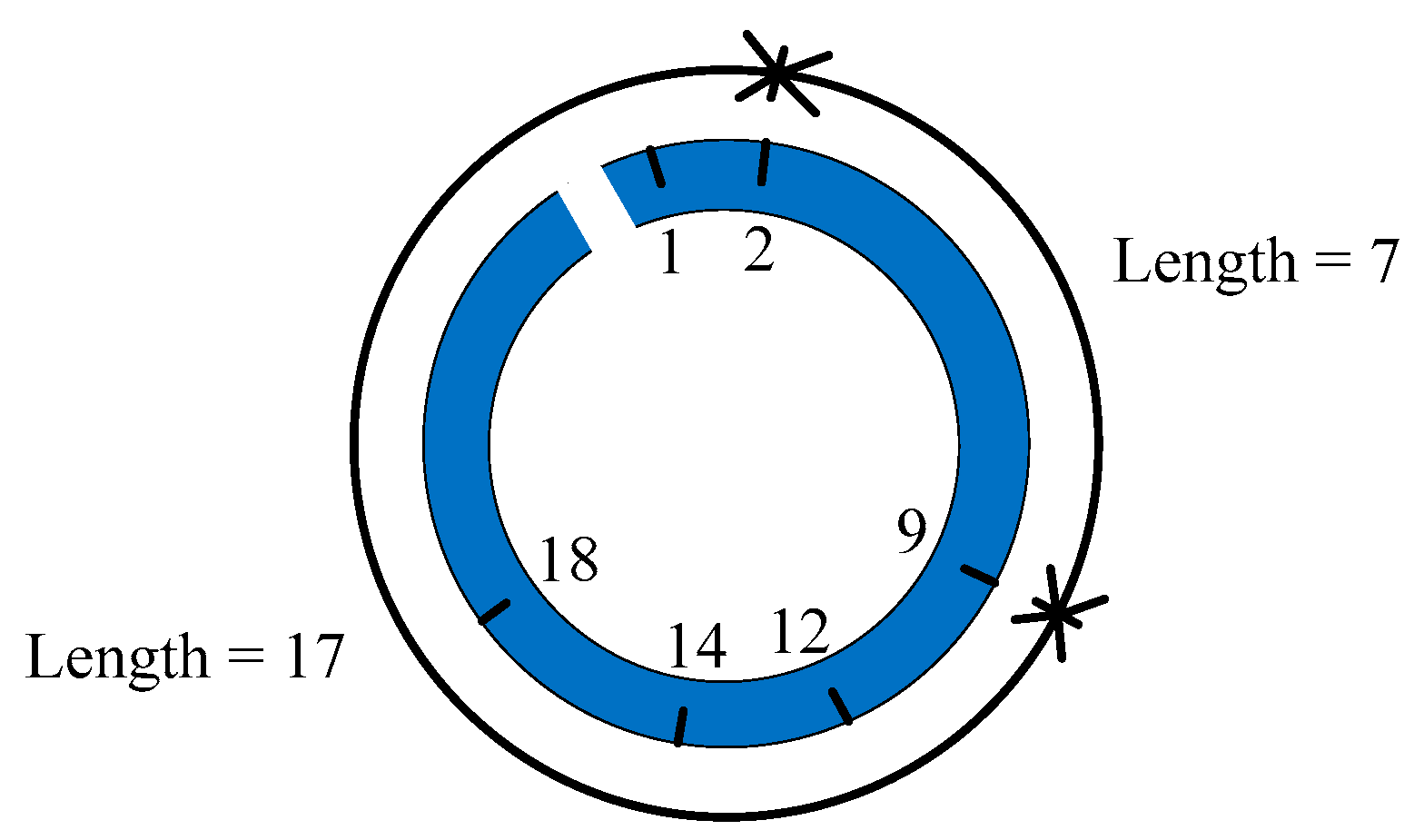
Next, we briefly introduce the concept of the circular sparse ruler. A
L-length circular sparse ruler can be viewed as a ruler with only
marks which is less than
L, but it is also able to measure all the length between 1 and
L. Define the
marks as
, and their difference set
, where
is the modulus operator. A set
is a circular sparse ruler if its difference set
. An example of the circular sparse ruler is given in
Figure 4, where the marks are
and the measurement range is
. Although there is no mark 7 and 17 on the sparse ruler, length 7 and 17 can be measured using mark 2 and 9.
The definition of difference set of circular sparse ruler
can be rewritten as
, where
and
. That is, if the difference set of the sampling pattern of MCS includes the set
, then each column vector of matrix
contains at least one non-zero element 1. Combined with the fact that the row vector of
has only one non-zero element 1, the matrix
will have full column rank. Therefore, the sampling pattern design of the MCS can be viewed as a circular sparse ruler problem. Please note that circular sparse ruler uses the difference between two marks to measure any length between 1 and
. If we want to measure length 1 to length
, then at least one pair of marks, or cosets, should have length 1 difference, or
time difference. Further, to obtain the strongest compression rate, we would like to minimize the cardinality of
, which can be viewed as a minimal circular sparse ruler problem. Then finally, let
and
denote the
i+2-th and
i-th coset, respectively.
should be greater than
because the S/H in
Figure 2 can only temporarily store one sample and the minimal sampling interval of ADC is
. Therefore, the design of sampling pattern turns into the following optimization problem:
where the sampling pattern
.
6. Simulation Results
This section evaluates the spectrum-sensing performance of the proposed single-channel sub-Nyquist sampling by performing several numerical simulations. In practice, an antenna is used to receive the Radio Frequency (RF) signal, and a band-pass filter is utilized to filter the out-of-band noise and interference. Subsequently, the RF signal is demodulated to baseband signal using a mixer. Finally, the Local Oscillator (LO) signal mixed in the demodulated signal is filtered out using a low-pass filter. Since the receiver front-end circuit is not the focus of this paper, we assume that the proposed single-channel sub-Nyquist sampling directly deals with the demodulated signal output from the low-pass filter in
Figure 2. Quadrature Phase-Shift Keying (QPSK) signal is used as the test signal, and it is generated by the following model:
where
is the number of primary users,
is the number of random bits,
and
are random bit streams,
is the pulse-shaping function,
is the symbol duration,
is the carrier frequency of the
k-th primary user, and
is the additive white Gaussian noise. Simulation parameters are set as follows:
The bandwidth of primary user is set as . The carrier frequency of primary user is randomly chosen from the center frequency of 40 channels. The pulse-shaping function is the root-raised cosine with roll-over factor 0.1. and are generated from pseudo-random binary sequence generator.
Additive white Gaussian noise , where is fixed to 1 and in Equation (34) is scaled to a certain SNR level.
The minimum modulation bandwidth of primary user is set as .
To simulate the mismatch behavior of parallel MCS, the clock timing skew is set as 2% of the Nyquist sampling interval . The offset and gain mismatch are set as 2% and 2% of maximum amplitude of signal, respectively.
The parameters of log-normal shadowing in Equation (2) are set as follows: reference distance , the path loss at the reference point , the path loss exponent , the Gaussian random variable , the distance between the primary user and the cognitive radio device . In addition, primary users are passed through Rayleigh channels with .
In the second and third numerical simulation, 200 trials are performed, and averaged results are shown.
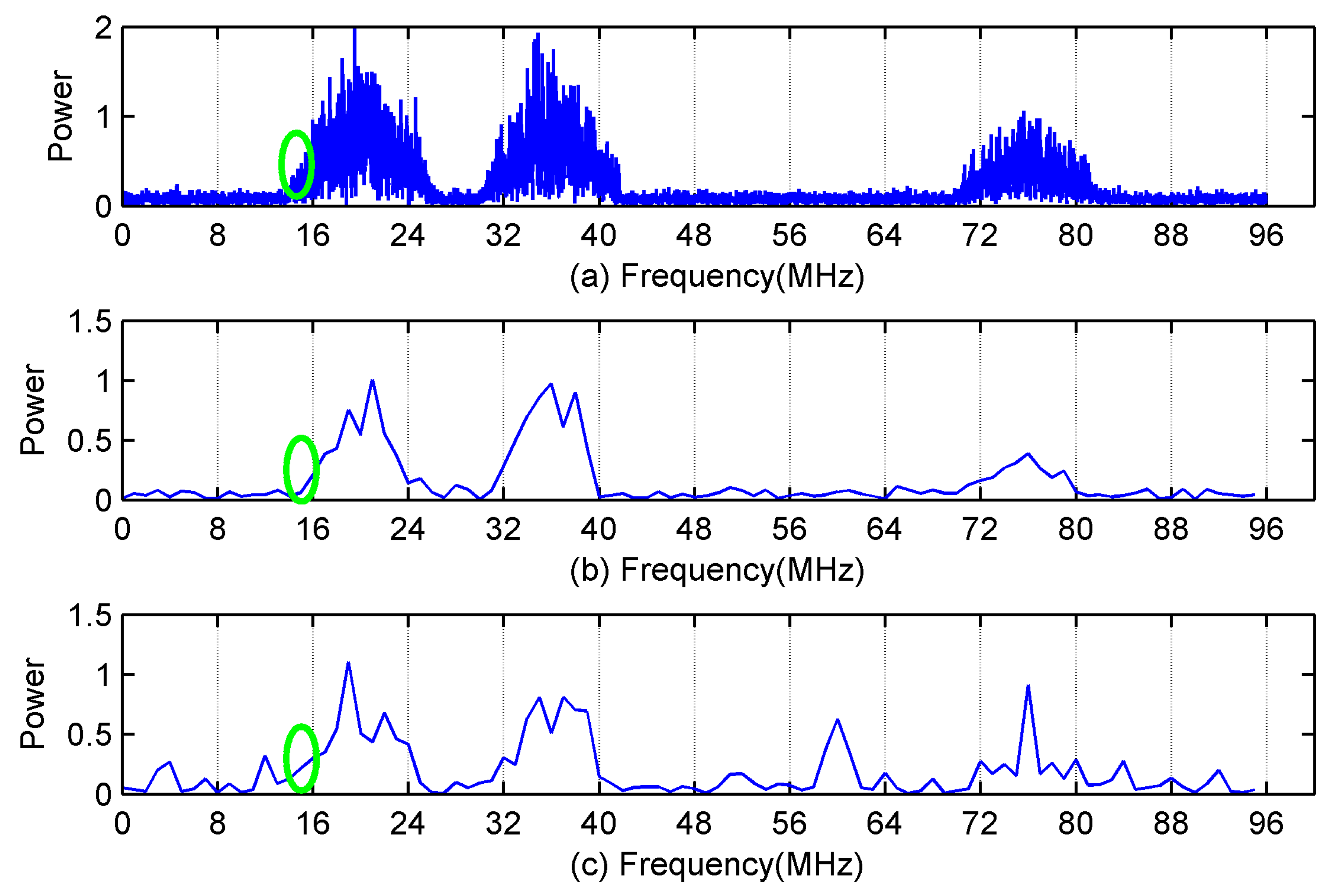
In the first simulation, we test the feasibility of spectrum sensing using power spectrum at partial frequency bins. To show the estimated frequency-smoothed power spectrum clearly, we only observed 12 of these 40 channels. In the following two simulations, 32 of these 40 channels are observed. The parameters of MCS are set as
,
and the sampling pattern is
. The number of active primary users is set as
. The SNR of the test signal is set as 10 dB, and the acquisition time is set as 64 μS.
Figure 5a shows the original power spectrum of the test signal.
Figure 5b,c show the estimated frequency-smoothed power spectrum at partial frequency bins using the proposed serial MCS and the traditional parallel MCS, respectively.
Figure 5b reflects the profile information of the original power spectrum because frequency-smoothed cross-periodogram is used in Equation (24). Using the frequency-smoothed cross-periodogram is equivalent to taking a weighted average of the power spectrum in the frequency-smoothing window. The weight value in the middle of the window is the largest and decreases toward each side. The profile information of the original power spectrum is sufficient for the spectrum-sensing module to detect primary users. It is unnecessary to estimate power spectrum at all frequency bins because the power spectrum at two frequency bins within the frequency-smoothing window are highly correlated. The proposed efficient spectrum-sensing algorithm exploits the frequency-smoothing characteristic to reduce the computational complexity.
On the other hand, as shown in
Figure 5c, mismatches among sub-ADCs in traditional parallel MCS cause large errors in the estimated power spectrum. Although these errors do not exist after calibration, the calibration will add a lot of additional burden to the system. Therefore, the proposed serial MCS combined with the efficient spectrum-sensing algorithm is a better choice.
In practice, the primary user signal arrives at the antenna of the cognitive radio device through multiple paths. Due to the different arrival time, the superposition of these signals will result in the distortion of the original signal. Rayleigh distribution is a model that can be used to describe this form of fading when multipath propagation exists. Rayleigh fading will result in Doppler shift, which equivalents to the expansion in the frequency domain. As shown in the green circle of
Figure 5, although the baseband width of the primary user of the third channel is 8 MHz, the Doppler shift caused by the multipath effect causes the energy of the third channel leak into the second channel. As a result, cognitive radio devices may mistakenly regard the primary user of the second channel also exists. In addition, Log-normal Shadowing significantly attenuates the amplitude of signal. When the amplitude of primary user signal is close to that of noise, the proposed method is difficult to detect the presence of the primary user. Cooperative spectrum sensing based on decision fusion can efficiently solve the shadow fading problem.
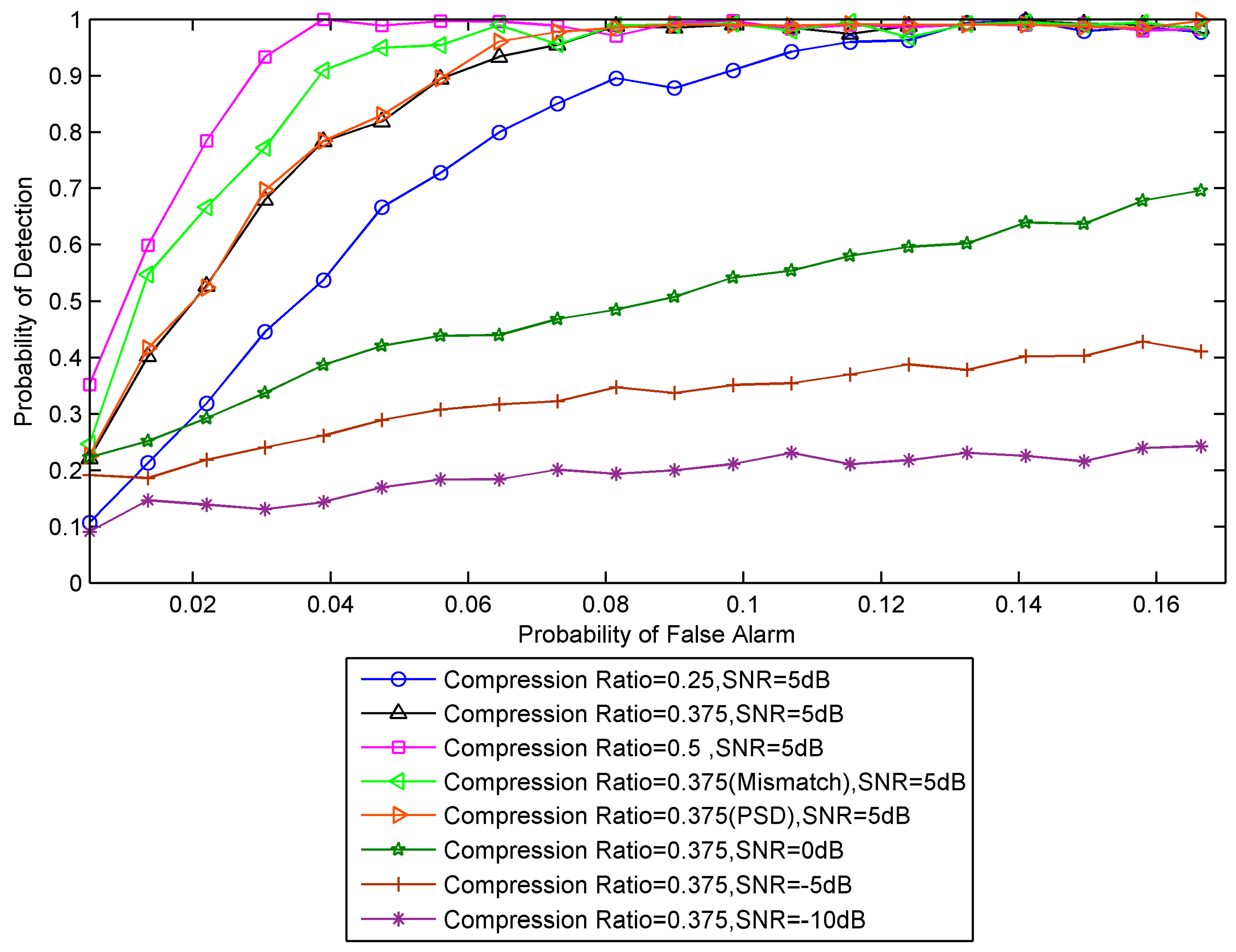
In the second simulation, we evaluate spectrum-sensing performance in terms of different compression ratio. 32 channels are observed in this simulation. Its bandwidth and Nyquist sampling rate are 256 MHz and 512 MSPS (Mega-Samples Per Second), respectively. We consider several SNRs and they are 5 dB, 0 dB, −5 dB and −10 dB. The periodicity of the sampling instants is set as in MCS. Several compression ratio are considered, and they are 0.25, 0.375 and 0.5. The sampling pattern for compression ratio 0.25 is , and the sampling rate requirement for ADC is 128 MSPS. The sampling pattern for compression ratio 0.375 is , and the sampling rate requirement for ADC is 192 MSPS. The sampling pattern for compression ratio 0.5 is , and the sampling rate requirement for ADC is 256 MSPS. The number of active primary users is set as . The acquisition time is set as 64 μS.
Figure 6 shows the Receiver Operating Characteristic (ROC) curve of the detector for different compression ratios. It is noticed that spectrum-sensing performance under different compression ratios is different. The more compression, the worse the detection performance. The curve corresponding to ‘Compression Ratio = 0.375 (Mismatch)’ in
Figure 6 is spectrum-sensing performance based on the parallel MCS with mismatches. Please note that the detection performance of the parallel MCS is better than that of the proposed serial MCS. The reason is that the mismatch error component is mistakenly regarded as primary users. The curve corresponding to ‘Compression Ratio = 0.375 (PSD)’ in
Figure 6 is spectrum-sensing performance using the power spectrum at all frequency bins. The detection performance is slightly different from the detection performance using the power spectrum at partial frequency bins, while the later one reduces a large amount of computation.
Table 1 shows the reduced computational complexity. The proposed efficient spectrum-sensing algorithm uses the frequency-smoothed cyclic cross-periodogram to estimate the smoothed power spectrum. Since the power spectrum of the smoothed power spectrum at two adjacent frequency bins are highly correlated, it is not necessary to estimate the power spectrum at all frequency bins, which reduces the computational complexity of spectrum sensing.
In the third simulation, we evaluate spectrum-sensing performance in terms of different acquisition time. The proposed efficient spectrum-sensing algorithm requires the signal be stationary during the acquisition process. To consider the fast time-varying signal, the detection performance under short acquisition time condition is tested. The compression ratio is fixed to 0.375. Several acquisition time are considered, and they are 16 μS, 64 μS, and 128 μS. Other simulation parameters are the same with the second simulation.
As shown in
Figure 7, spectrum-sensing performance gradually improves as the SNR increases. When the SNR is greater than 5 dB, the proposed efficient spectrum-sensing algorithm exhibits a perfect detection performance. The shorter the acquisition time, the worse the spectrum-sensing performance. Short acquisition time means that the number of samples used to calculate frequency-smoothed cross-periodogram in Equation (24) is small. Thus, the estimate accuracy of the frequency-smoothed cross-periodogram is affected. Ultimately, spectrum-sensing performance is influenced. In the case that the acquisition time is 16 μS, it is guaranteed that all primary users and spectrum holes can be detected with high probability when the SNR is higher than 5 dB.
The curve corresponding to ‘Acquisition Time = 64 μS (PSD)’ is spectrum-sensing performance using power spectrum at all frequency bins. It is shown that spectrum-sensing performance based on power spectrum at all frequency bins has little improvement. Therefore, spectrum sensing using power spectrum at partial frequency bins is preferable since it reduces a large amount of computation.
Table 2 compares the required computational complexity between the conventional method and the proposed method. The reason for the reduction of computational complexity is the same as that of the second simulation.
Compared with the detection performance, the false alarm probability is also very important. False alarm probability determines how many spectrum holes are available to secondary users. The curve corresponding to ‘Acquisition Time = 64 μS (Mismatch)’ is spectrum-sensing performance using the traditional parallel MCS with mismatches. Mismatches have little influence on the detection performance as shown in
Figure 7a, while they have severe influence on the false alarm probability as shown in
Figure 7b. The false alarm probability of the proposed serial MCS gradually decreases to 0 as the SNR increases. However, the false alarm probability of the traditional parallel MCS does not tend to zero even if the SNR is high. As shown in
Figure 7b, all spectral holes can be detected with high probability when the SNR is higher than 8dB for serial MCS.


