Dense RGB-D SLAM with Multiple Cameras


Abstract
:1. Introduction
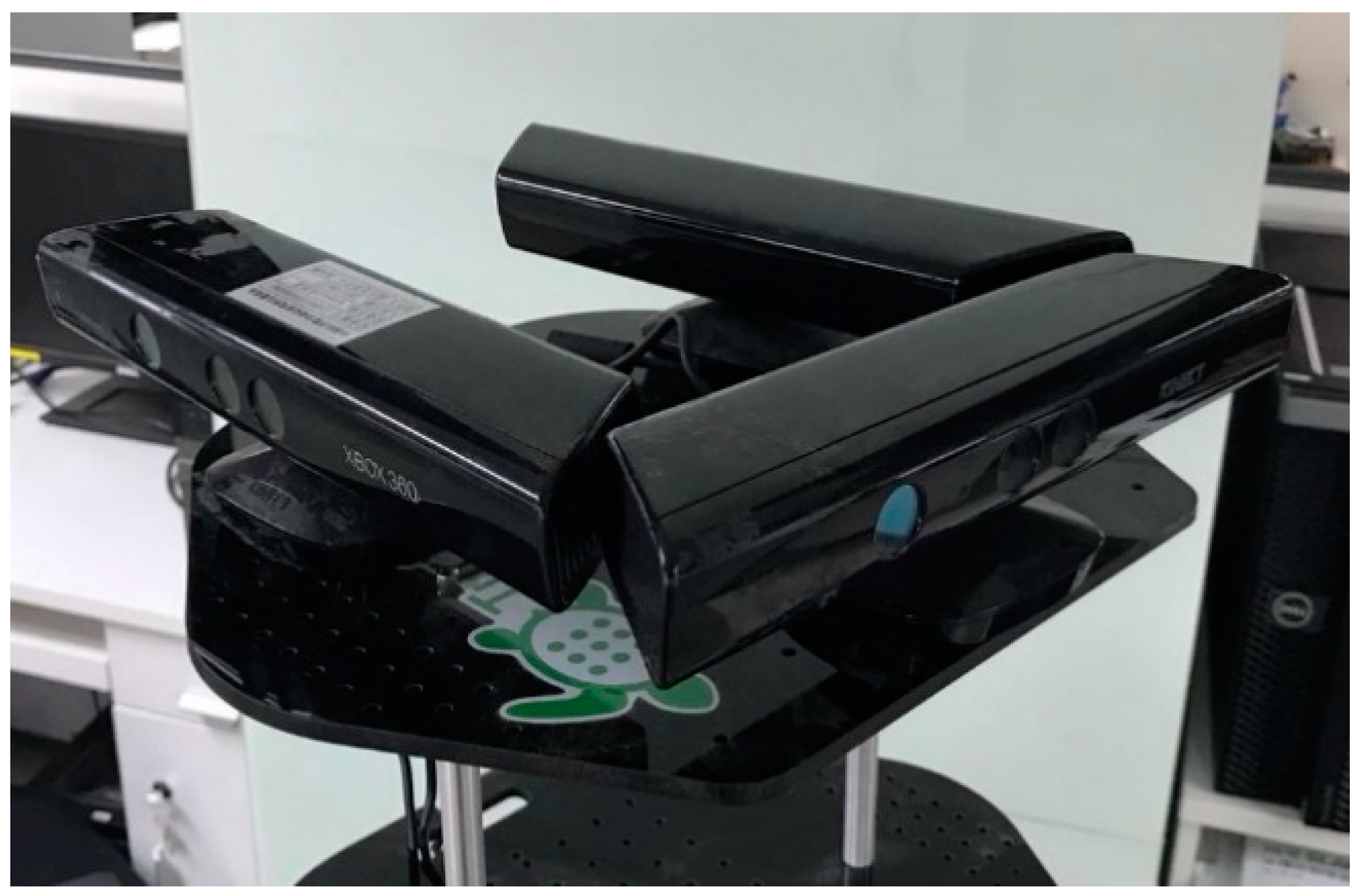
- Two kinds of extrinsic calibration methods for three-Kinect system are proposed, one is suitable for system with IMU using an improved hand–eye calibration method, the other for pure visual SLAM without any other auxiliary sensors.
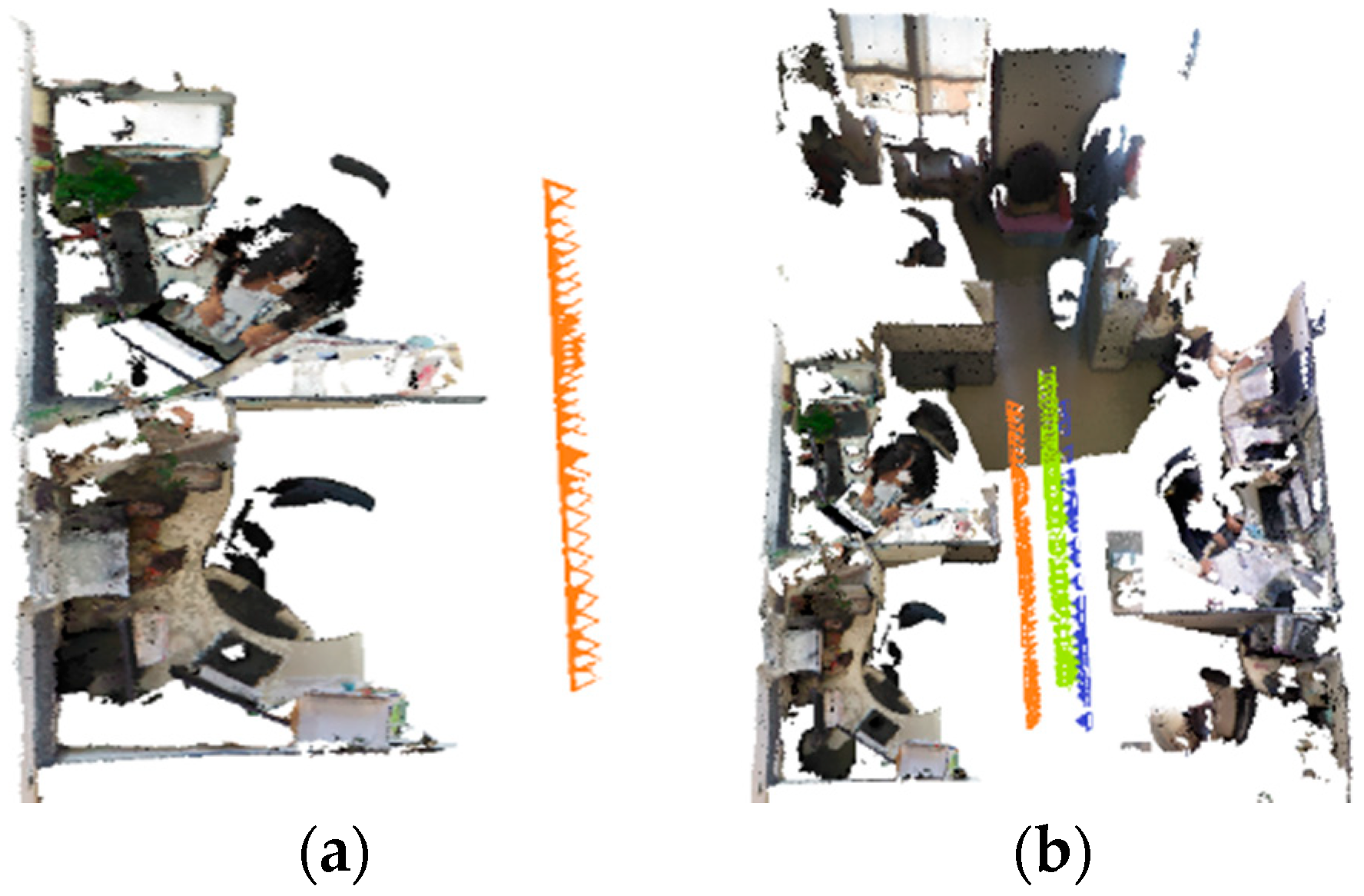
- We extend the state-of-the-art ElasticFusion [20] to a multi-camera system to get a better dense RGB-D SLAM.
2. Extrinsic Calibration of Multiple Cameras
2.1. Odometer-Based Extrinsic Calibration
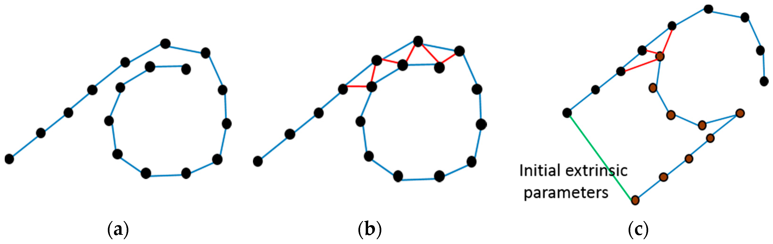
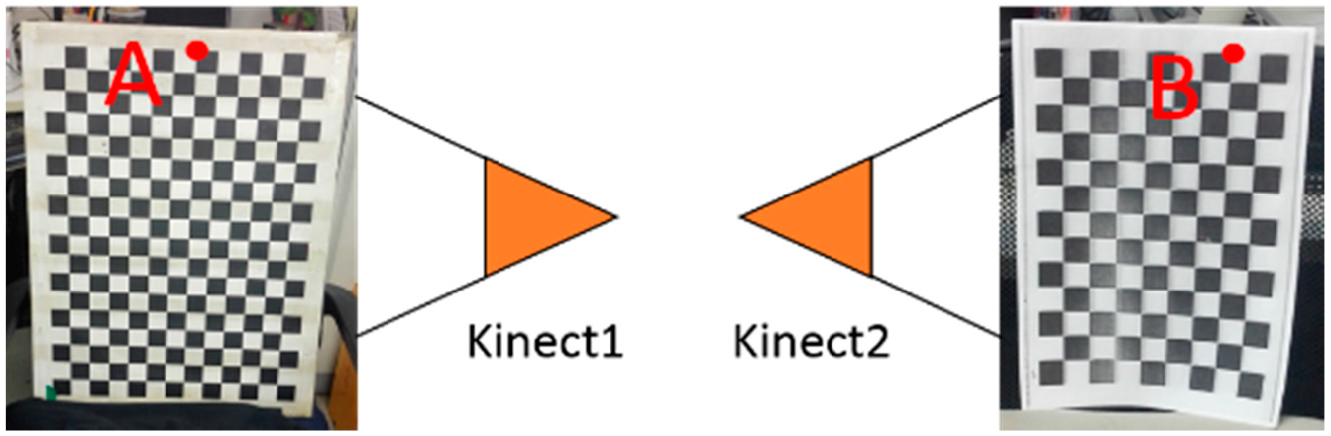
2.2. SLAM-Based Extrinsic Calibration
3. Multi-Camera RGB-D SLAM
3.1. Tracking
3.2. Mapping
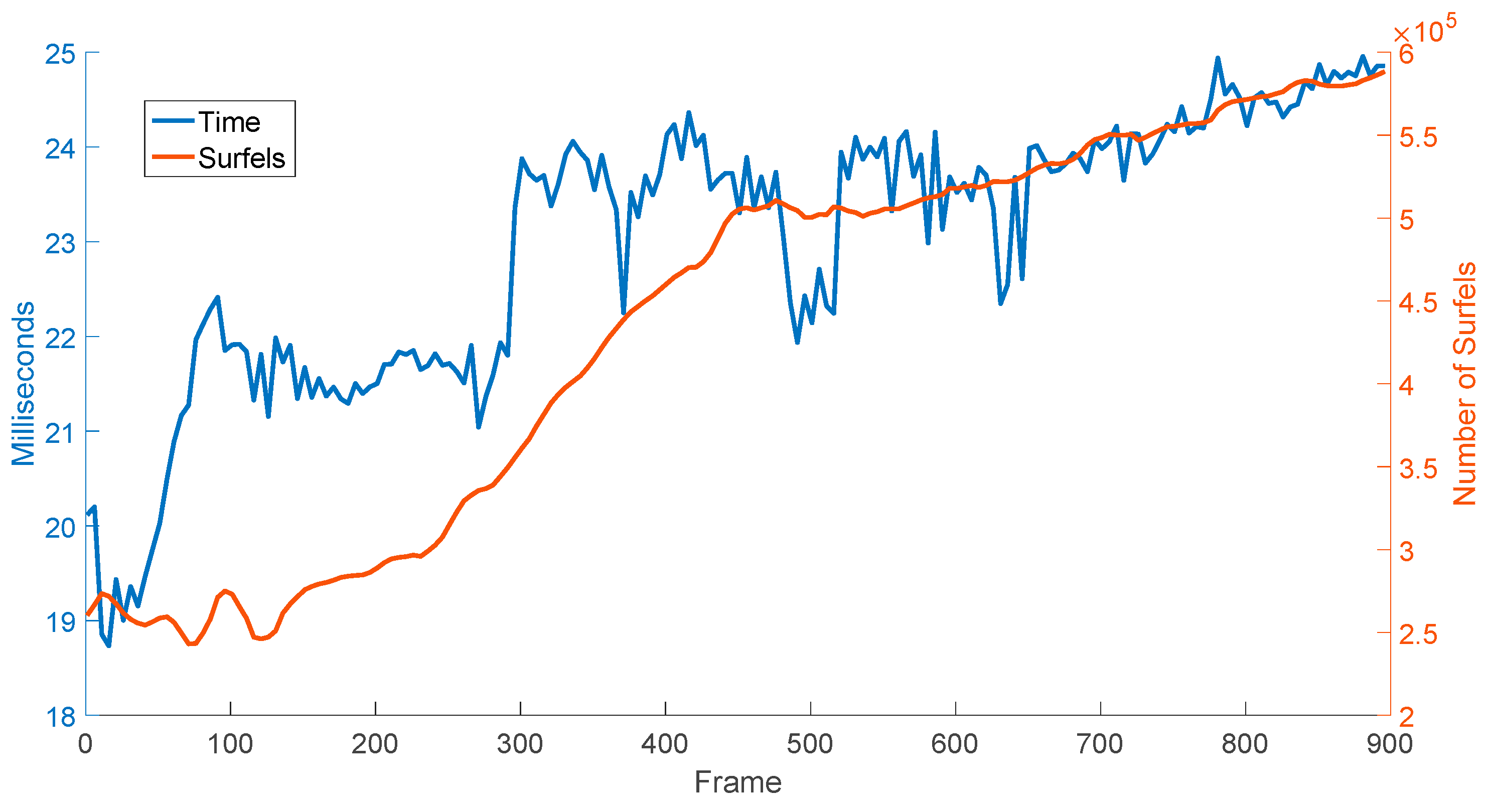
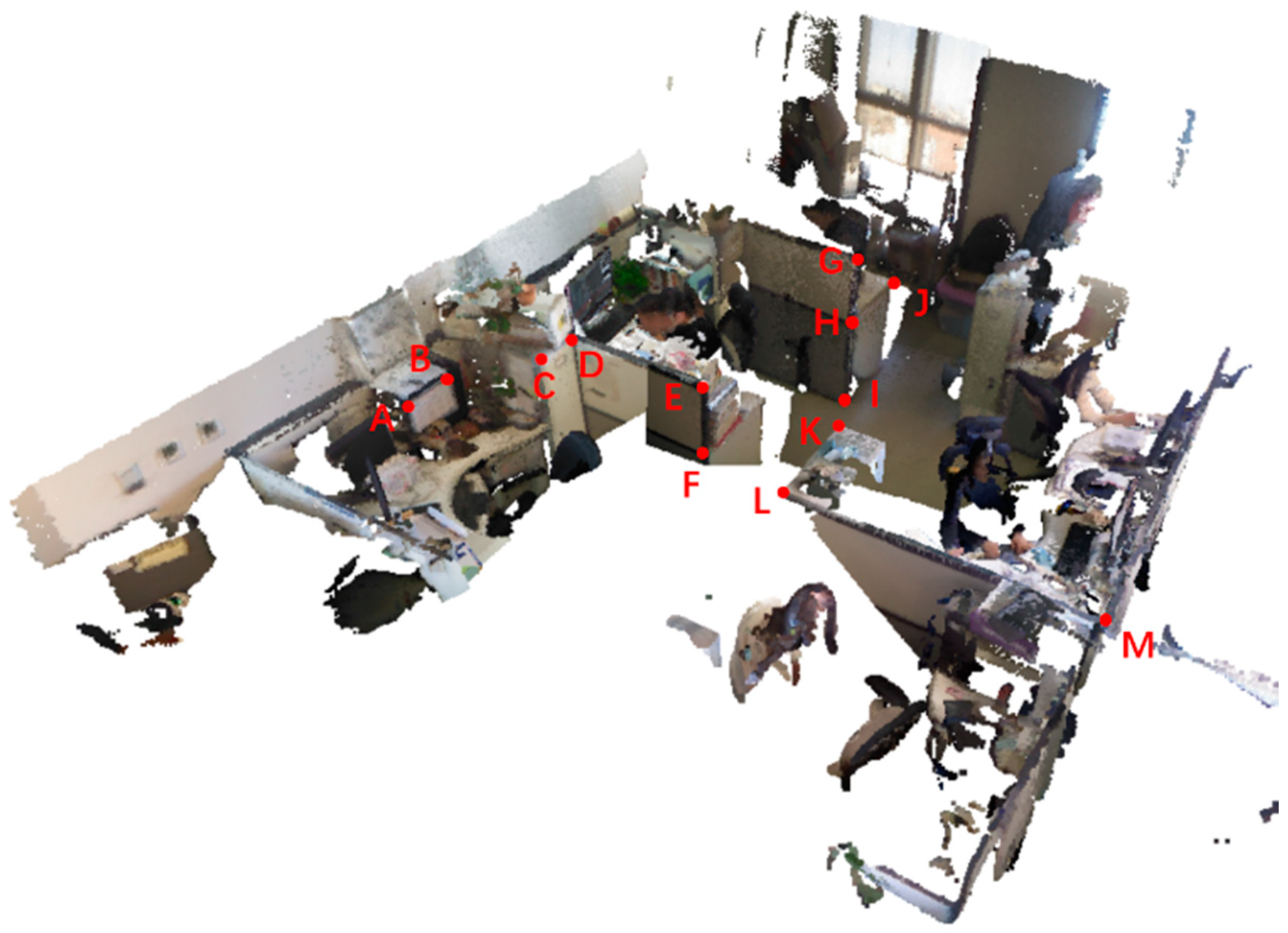
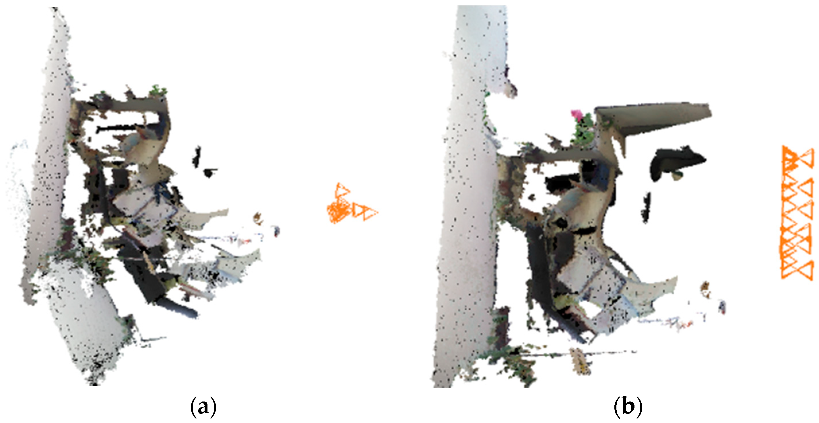
4. Experiment
5. Conclusions
Author Contributions
Funding
Conflicts of Interest
References
- Villena-Martínez, V.; Fuster-Guilló, A.; Azorín-López, J.; Saval-Calvo, M.; Mora-Pascual, J.; Garcia-Rodriguez, J.; Garcia-Garcia, A. A quantitative comparison of calibration methods for RGB-D sensors using different technologies. Sensors 2017, 17, 243. [Google Scholar] [CrossRef] [PubMed]
- Rufli, M.; Scaramuzza, D.; Siegwart, R. Automatic detection of checkerboards on blurred and distorted images. In Proceedings of the IEEE/RSJ International Conference on Intelligent Robots and Systems, Nice, France, 22–26 September 2008; pp. 3121–3126. [Google Scholar]
- Li, B.; Heng, L.; Koser, K.; Pollefeys, M. A multiple-camera system calibration toolbox using a feature descriptor-based calibration pattern. In Proceedings of the IEEE/RSJ International Conference on Intelligent Robots and Systems, Tokyo, Japan, 3–7 November 2013; pp. 1301–1307. [Google Scholar]
- Su, P.C.; Shen, J.; Xu, W.; Cheung, S.C.; Luo, Y. A fast and robust extrinsic calibration for RGB-D camera networks. Sensors 2018, 18, 235. [Google Scholar] [CrossRef] [PubMed]
- Tsai, R.Y.; Lenz, R.K. A new technique for fully autonomous and efficient 3D robotics hand/eye calibration. IEEE Trans. Robotics Autom. 1989, 5, 345–358. [Google Scholar] [CrossRef]
- Chang, Y.L.; Aggarwal, J.K. Calibrating a mobile camera’s extrinsic parameters with respect to its platform. In Proceedings of the 1991 IEEE International Symposium on Intelligent Control, Arlington, VA, USA, 13–15 August 1991; pp. 443–448. [Google Scholar]
- Guo, C.X.; Mirzaei, F.M.; Roumeliotis, S.I. An analytical least-squares solution to the odometer-camera extrinsic calibration problem. In Proceedings of the 2012 IEEE International Conference on Robotics and Automation (ICRA), Saint Paul, MN, USA, 14–18 May 2012; pp. 3962–3968. [Google Scholar]
- Heng, L.; Li, B.; Pollefeys, M. Camodocal: Automatic intrinsic and extrinsic calibration of a rig with multiple generic cameras and odometry. In Proceedings of the 2013 IEEE/RSJ International Conference on Intelligent Robots and Systems (IROS), Tokyo, Japan, 3–7 November 2013; pp. 1793–1800. [Google Scholar]
- Esquivel, S.; Woelk, F.; Koch, R. Calibration of a multi-camera rig from non-overlapping views. In Proceedings of the DAGM Symposium on Pattern Recognition, Heidelberg, Germany, 12–14 September 2007. [Google Scholar]
- Carrera, G.; Angeli, A.; Davison, A.J. SLAM-based automatic extrinsic calibration of a multi-camera rig. In Proceedings of the 2011 IEEE International Conference on Robotics and Automation (ICRA), Shanghai, China, 9–13 May 2011; pp. 2652–2659. [Google Scholar]
- Di, K.; Zhao, Q.; Wan, W.; Wang, Y.; Gao, Y. RGB-D SLAM based on extended bundle adjustment with 2D and 3D information. Sensors 2016, 16, 1285. [Google Scholar] [CrossRef] [PubMed]
- Tang, S.; Zhu, Q.; Chen, W.; Darwish, W.; Wu, B.; Hu, H.; Chen, M. Enhanced RGB-D mapping method for detailed 3D indoor and outdoor modeling. Sensors 2016, 16, 1589. [Google Scholar] [CrossRef] [PubMed]
- Fu, X.; Zhu, F.; Wu, Q.; Sun, Y.; Lu, R.; Yang, R. Real-time large-scale dense mapping with surfels. Sensors 2018, 18, 1493. [Google Scholar] [CrossRef] [PubMed]
- Huang, A.S.; Bachrach, A.; Henry, P.; Krainin, M.; Maturana, D.; Fox, D.; Roy, N. Visual odometry and mapping for autonomous flight using an RGB-D camera. In Robotics Research; Springer: Cham, Switzerland, 2016; pp. 235–252. [Google Scholar]
- Hartley, R.; Zisserman, A. Multiple View Geometry in Computer Vision; Cambridge University Press: Cambridge, UK, 2000. [Google Scholar]
- Kaess, M.; Dellaert, F. Visual Slam with a Multi-Camera Rig; Georgia Institute of Technology: Atlanta, GA, USA, 2006. [Google Scholar]
- Sola, J.; Monin, A.; Devy, M.; Vidal-Calleja, T. Fusing monocular information in multicamera SLAM. IEEE Trans. Robot. 2018, 24, 958–968. [Google Scholar] [CrossRef]
- Urban, S.; Hinz, S. MultiCol-SLAM-A Modular Real-Time Multi-Camera SLAM System. arXiv, 2016; arXiv:1610.07336. [Google Scholar]
- Alexiadis, D.S.; Chatzitofis, A.; Zioulis, N.; Zoidi, O.; Louizis, G.; Zarpalas, D.; Daras, P. An integrated platform for live 3D human reconstruction and motion capturing. IEEE Trans. Circuits Syst. Video Technol. 2017, 27, 798–813. [Google Scholar] [CrossRef]
- Whelan, T.; Leutenegger, S.; Salas-Moreno, R.F.; Glocker, B.; Davison, A.J. ElasticFusion: Dense SLAM without a pose graph. In Proceedings of the Robotics: Science and Systems, Rome, Italy, 13–17 July 2015. [Google Scholar]
- Newcombe, R.A.; Izadi, S.; Hilliges, O.; Molyneaux, D.; Kim, D.; Davison, A.J.; Kohi, P.; Shotton, J.; Hodges, S.; Fitzgibbon, A. KinectFusion: Real-time dense surface mapping and tracking. In Proceedings of the 2011 10th IEEE International Symposium on Mixed and Augmented Reality (ISMAR), Basel, Switzerland, 26–29 October 2011; pp. 127–136. [Google Scholar]
- Blais, G.; Levine, M.D. Registering multiview range data to create 3D computer objects. IEEE Trans. Pattern Anal. Mach. Intell. 1995, 17, 820–824. [Google Scholar] [CrossRef]
- Arun, K.S.; Huang, T.S.; Blostein, S.D. Least-squares fitting of two 3-D point sets. IEEE Trans. Pattern Anal. Mach. Intell. 1987, 698–700. [Google Scholar] [CrossRef]
- Kahler, O.; Prisacariu, V.A.; Ren, C.Y.; Sun, X.; Torr, P.; Murray, D. Very High Frame Rate Volumetric Integration of Depth Images on Mobile Devices. IEEE Trans. Vis. Comput. Graph. 2015, 21, 1241–1250. [Google Scholar] [CrossRef] [PubMed]


| Sequence | Ground Truth | Odometer Calib | SLAM Calib | Odo + SLAM Calib |
|---|---|---|---|---|
| 1 | 2.510 m | 2.489 m | 2.481 m | 2.490 m |
| 2 | 1.969 m | 1.953 m | 1.940 m | 1.955 m |
| Line Segment | Length in Our Reconstructed Model | Length in the Reconstructed Model by InfiniTAM | Actual Length |
|---|---|---|---|
| AB | 28.64 cm | 27.51 cm | 29.50 cm |
| CD | 26.37 cm | 27.02 cm | 27.00 cm |
| EF | 44.80 cm | 44.06 cm | 44.30 cm |
| GI | 121.13 cm | 118.48 cm | 118.50 cm |
| HJ | 62.84 cm | 61.82 cm | 62.10 cm |
| KL | 63.44 cm | 61.20 cm | 62.30 cm |
| LM | 168.37 cm | 172.87 cm | 170.50 cm |
| RMSE | 1.55 cm | 1.34 cm | / |
© 2018 by the authors. Licensee MDPI, Basel, Switzerland. This article is an open access article distributed under the terms and conditions of the Creative Commons Attribution (CC BY) license (http://creativecommons.org/licenses/by/4.0/).
Share and Cite
Meng, X.; Gao, W.; Hu, Z. Dense RGB-D SLAM with Multiple Cameras. Sensors 2018, 18, 2118. https://doi.org/10.3390/s18072118
Meng X, Gao W, Hu Z. Dense RGB-D SLAM with Multiple Cameras. Sensors. 2018; 18(7):2118. https://doi.org/10.3390/s18072118
Chicago/Turabian StyleMeng, Xinrui, Wei Gao, and Zhanyi Hu. 2018. "Dense RGB-D SLAM with Multiple Cameras" Sensors 18, no. 7: 2118. https://doi.org/10.3390/s18072118
APA StyleMeng, X., Gao, W., & Hu, Z. (2018). Dense RGB-D SLAM with Multiple Cameras. Sensors, 18(7), 2118. https://doi.org/10.3390/s18072118