Single-Input and Multiple-Output Surface Acoustic Wave Sensing for Damage Quantification in Piezoelectric Sensors

Abstract
1. Introduction
1.1. Single Input and Multiple Output
1.2. Different Types of Transducers
1.3. Data Analysis and Evaluation Procedures
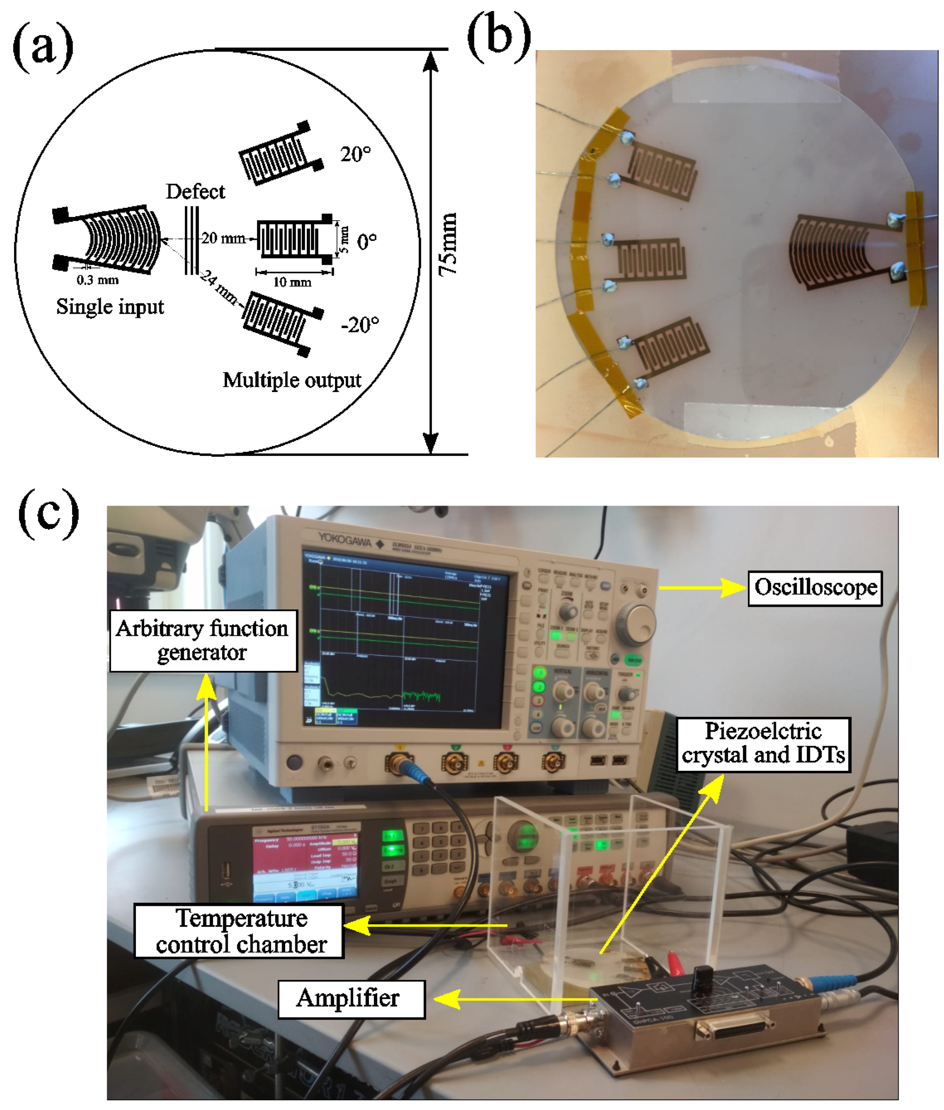
2. Interdigital Transducer Fabrication
3. Experimental Setup and Surface Flaw Generation
4. Algorithm for Damage Detection
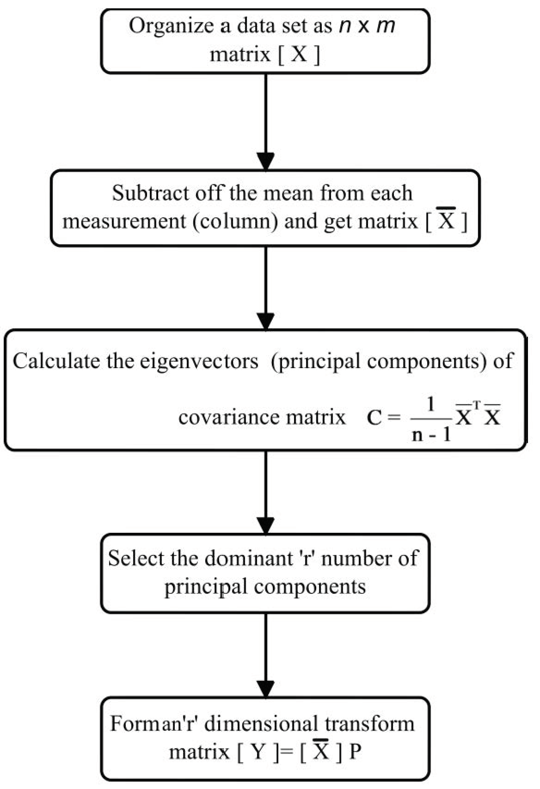
4.1. Principal Component Analysis
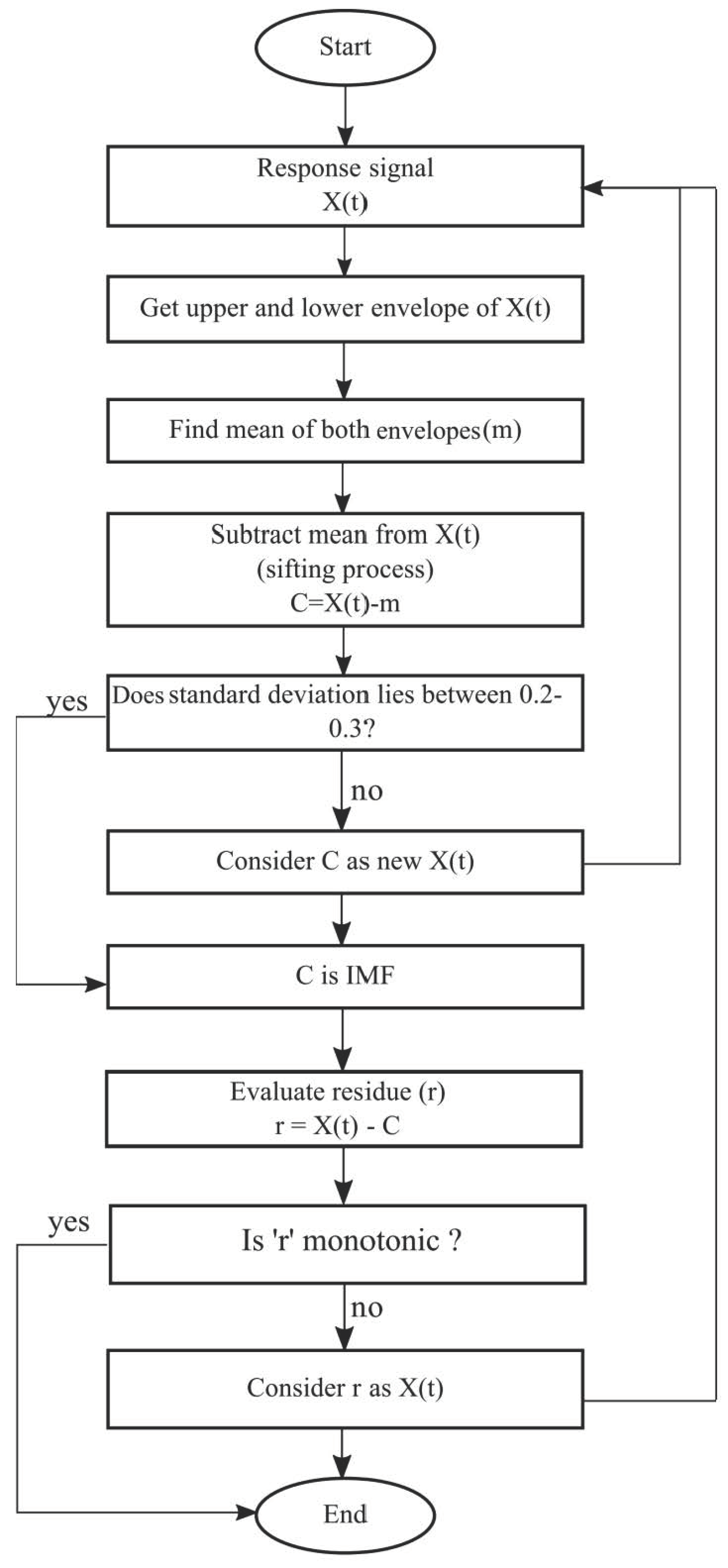
4.2. Empirical Mode Decomposition
4.3. Algorithm for Defect Detection
- (1)
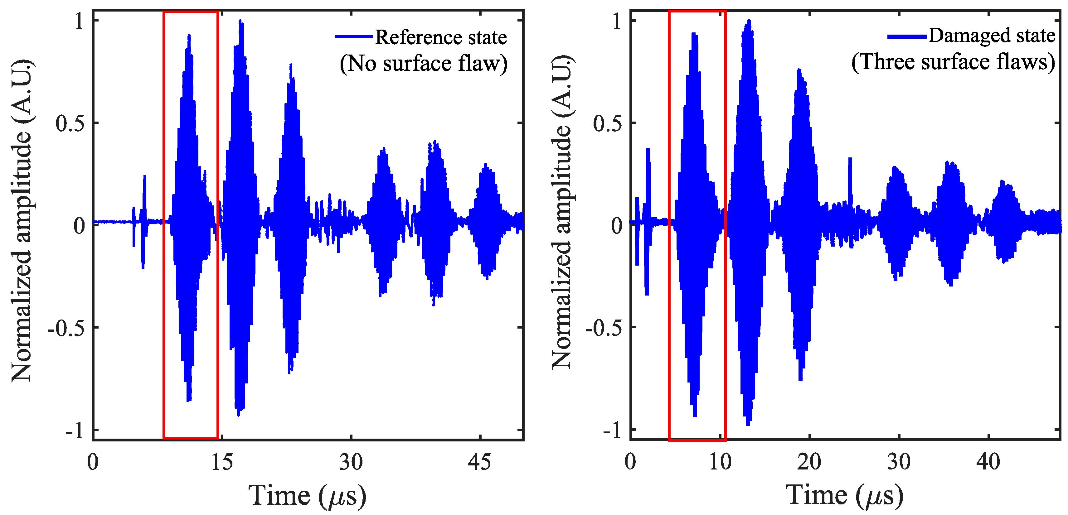
- Acquire the signal and form a response data matrix
- (2)
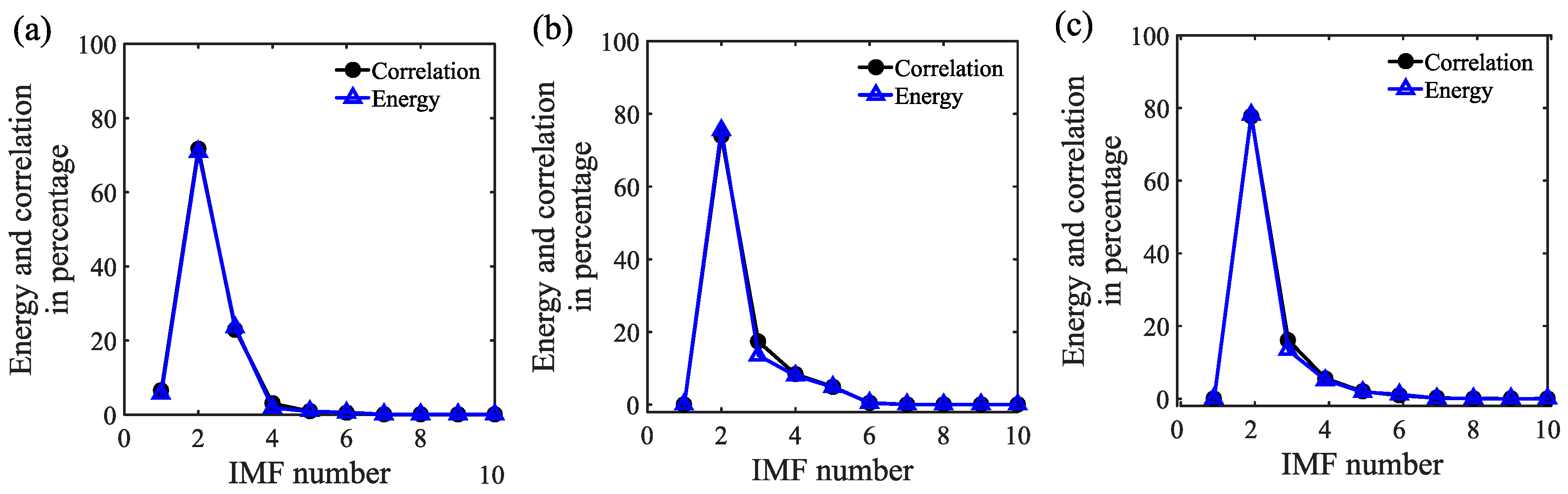
- With help of EMD get IMFs corresponding to each signal of response data matrix. Then after, select the dominant IMF for each signal with help of energy and correlation-based approach.
- (3)
- Process all the 2-dimensional combinations of response matrix by PCA and evaluate principal components (PCs) for each. Repeat the above process for baseline as well as damage states.
- (4)
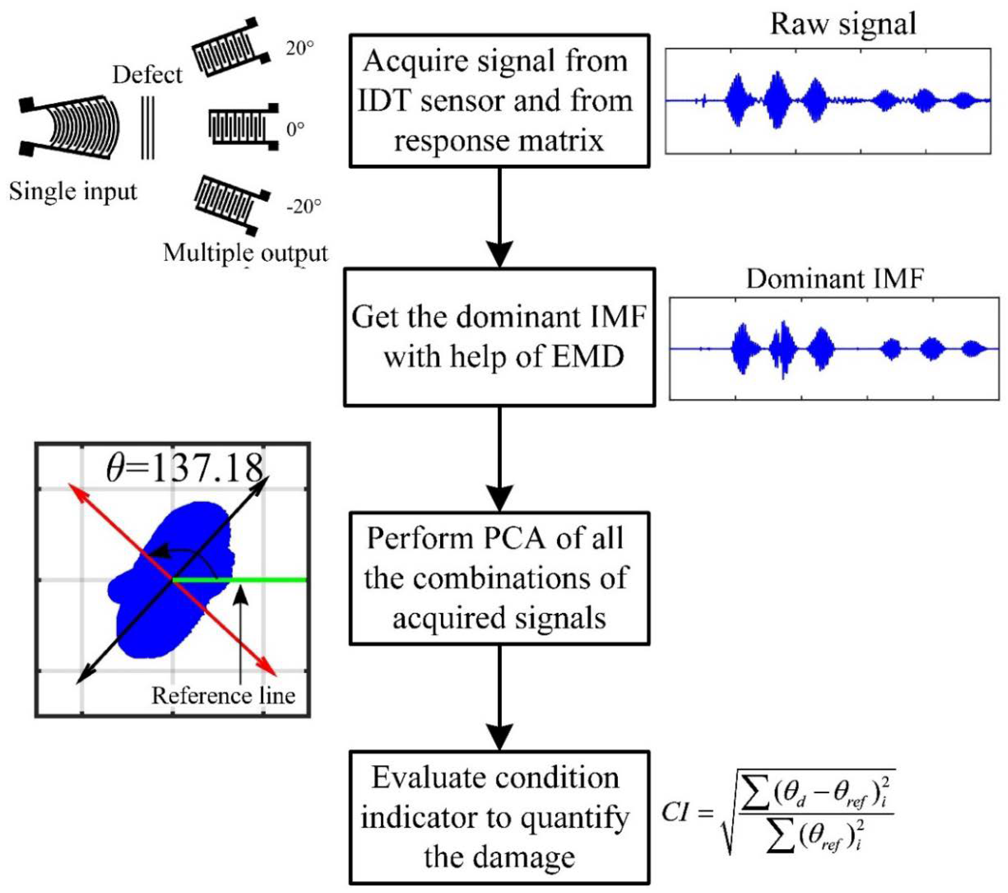
- Evaluate the condition indicator (CI) based on change in the angle of PCs. The detailed explanation of CI is in Section 5.2. The CI successfully segregates damage state from healthy state, it also quantifies the defect.
- (1)
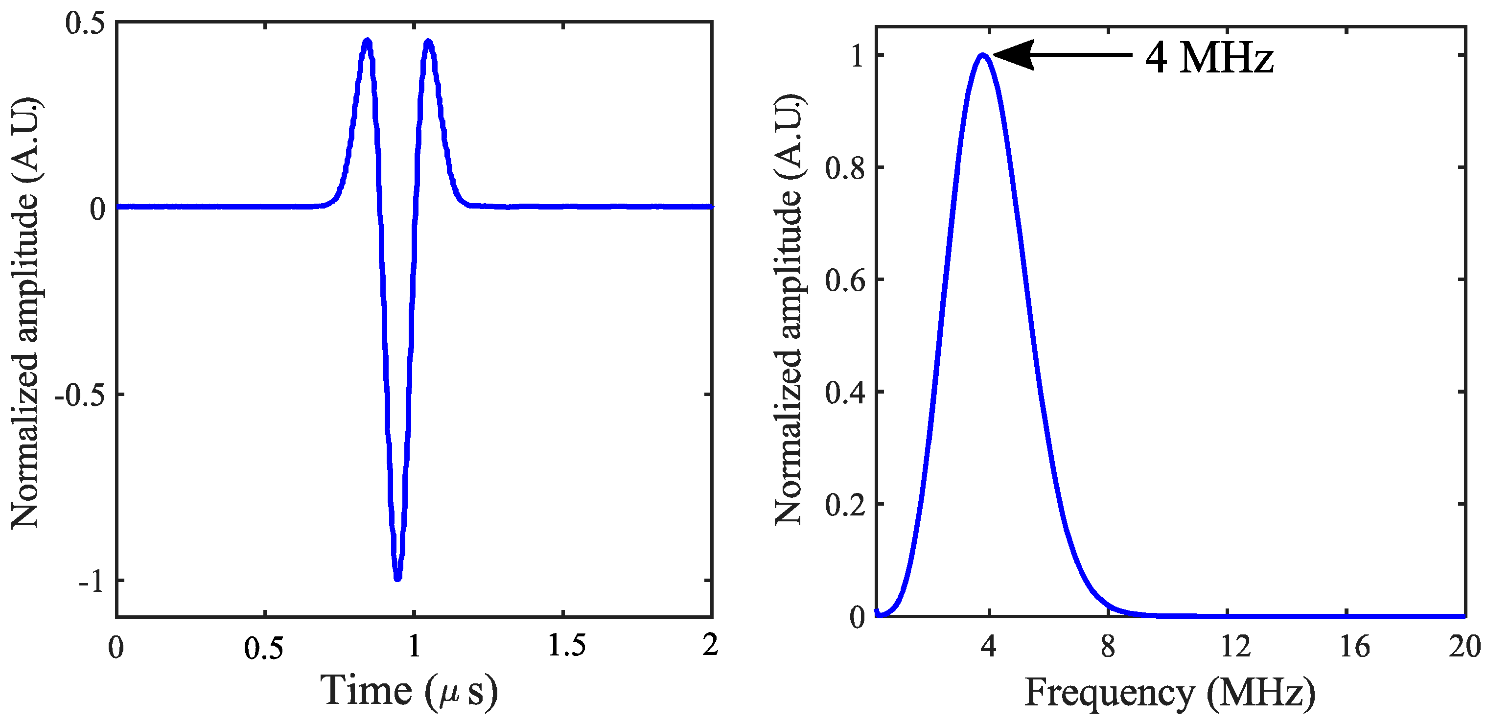
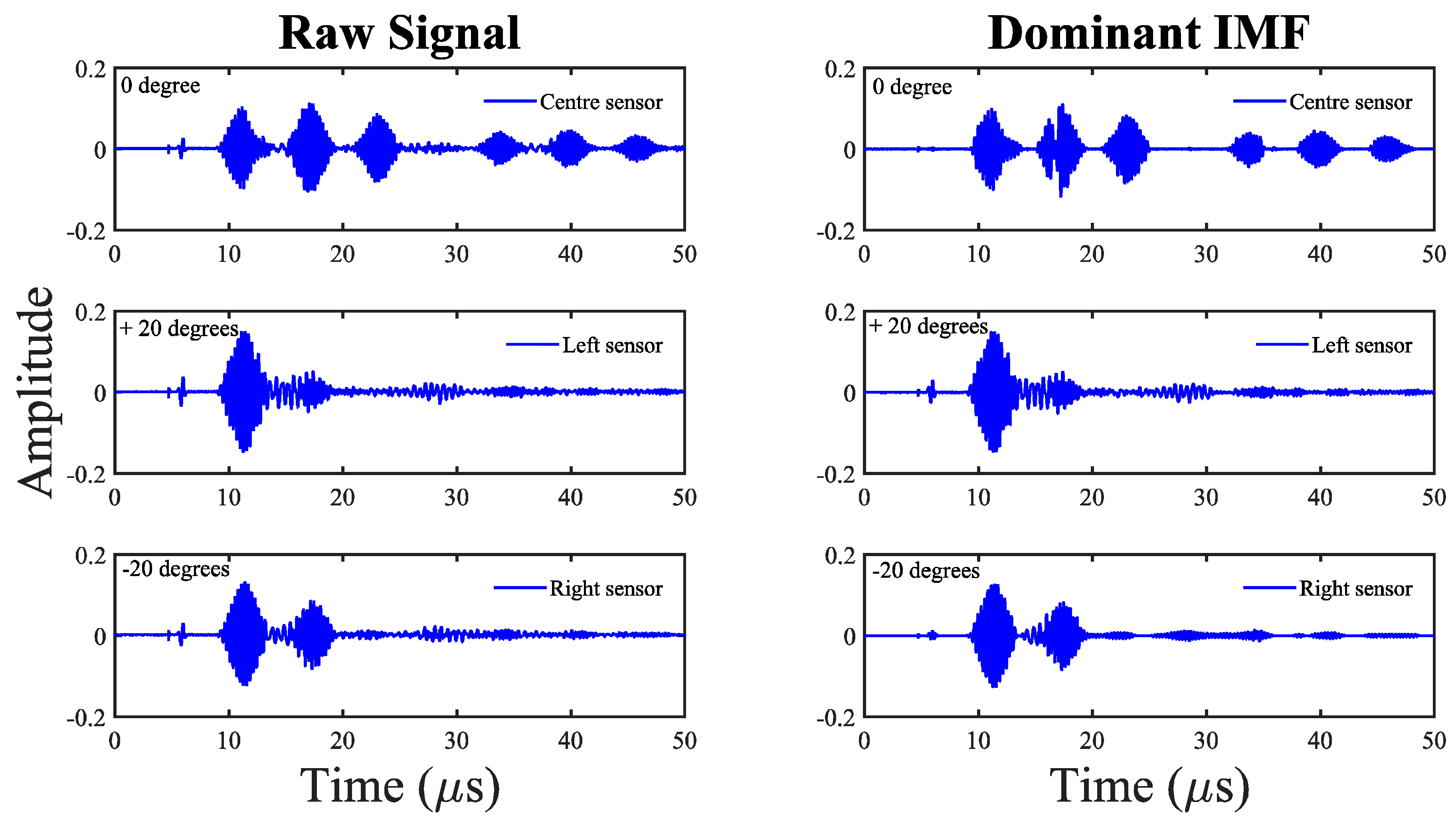
- The piezoelectric crystal is excited by a broadband pulse and the response is acquired by three IDT sensors mounted. The acquired data forms a response data matrix [A] of size N × 3, where N is total number of samples acquired, and the numeric 3 is due to three IDT sensors.The EMD of each column vector of matrix A will result in multiple IMFs corresponding to each:where m is the number of IMFs obtained after EMD and is a row vector.The next step is to calculate energy and correlation of each monocomponent IMF. The IMF corresponding to maximum correlation and energy is selected as the dominant IMF. In the present case, , the results for correlation are the same. Therefore, the second IMF is selected as the dominant IMF.
- (2)
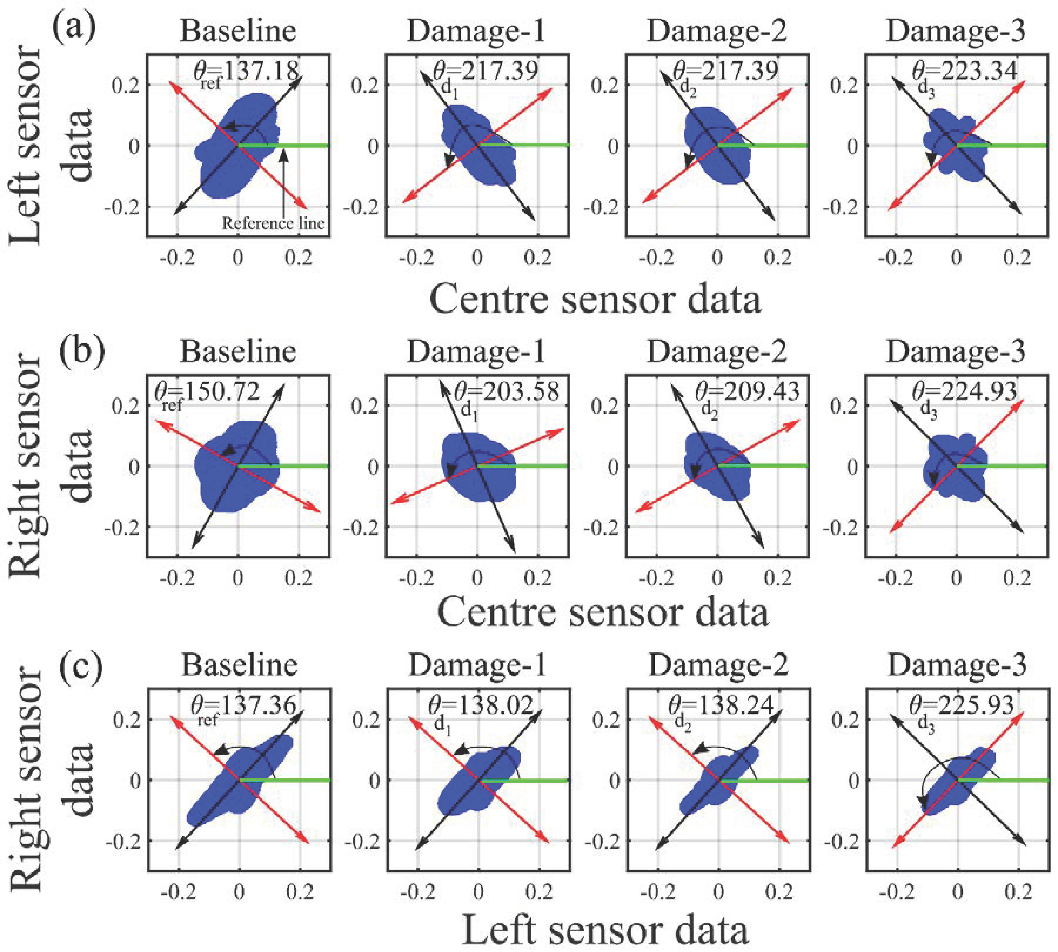
- In this step, we form all the possible two-dimensional combinations of the response matrix, and process it by PCA. Considering the response matrix of the current work, the three variables will lead to three two-dimensional combinations:where C-1, C-2 and C-3 represent combination one, combination two and combination three, respectively.The PCA of a combination will give its principal components and principal angles. The detailed explanation of PCA is given in Section 4.1. and are principal angles corresponding to a damaged case and healthy (reference) case, respectively.
- (3)
- Using the value of principal angle for reference and damaged cases, we evaluate the condition indicator (CI) proposed in the current work.where i is number of combinations of data.
5. Results and Discussion
5.1. Empirical Mode Decomposition of Response Signals
5.1.1. Energy-Based Approach
5.1.2. Correlation-Based Approach
5.2. Principal Component Analysis of Dominant Intrinsic Mode Functions
6. Conclusions
Author Contributions
Funding
Conflicts of Interest
List of Notations
| Acquired signal | |
| jth IMF of the signal | |
| T | total duration of the signal |
| N | the total number of data points |
| C | Covariance matrix |
| E | Residual error matrix |
| covariance between | |
| standard deviation of x(t) | |
| standard deviation of xj(t) | |
| Response matrix | |
| Zero mean response matrix | |
| XIMF | Matrix consisting of IMFs corresponding to response matrix |
| LiNbO3 | Lithium Niobate |
| Principal angle corresponding to reference case | |
| Principal angle corresponding to damage-i case |
References
- Fishler, E.; Haimovich, A.; Blum, R.; Chizhik, D.; Cimini, L.; Valenzuela, R. MIMO radar: An idea whose time has come. In Proceedings of the 2004 Radar Conference, Philadelphia, PA, USA, 29–29 April 2004; pp. 71–78. [Google Scholar]
- Carrascosa, P.C.; Stojanovic, M. Adaptive channel estimation and data detection for underwater acoustic MIMO–OFDM systems. IEEE OES 2010, 35, 635–646. [Google Scholar] [CrossRef]
- Heidemann, J.; Stojanovic, M.; Zorzi, M. Underwater sensor networks: Applications, advances and challenges. Philos. Trans. R. Soc. A 2012, 370, 158–175. [Google Scholar] [CrossRef] [PubMed]
- Zhang, X.; Xu, L.; Xu, L.; Xu, D. Direction of departure (DOD) and direction of arrival (DOA) estimation in MIMO radar with reduced-dimension MUSIC. IEEE Commun. Lett. 2010, 14, 1161–1163. [Google Scholar] [CrossRef]
- Duofang, C.; Baixiao, C.; Guodong, Q. Angle estimation using ESPRIT in MIMO radar. Electron. Lett. 2008, 44, 770–771. [Google Scholar] [CrossRef]
- Bencheikh, M.L.; Wang, Y. Joint DOD-DOA estimation using combined ESPRIT-MUSIC approach in MIMO radar. Electron. Lett. 2010, 46, 1081–1083. [Google Scholar] [CrossRef]
- Habib, A.; Ahmad, A.; Wagle, S.; Ahluwalia, B.S.; Melandsø, F.; Tiwari, A.K.; Mehta, D.S. Quantitative phase measurement for the damage detection in piezoelectric crystal using angularly placed multiple inter digital transducers. In Proceedings of the 2016 Ultrasonics Symposium (IUS), Tours, France, 18–21 September 2016; pp. 1–4. [Google Scholar]
- Rose, J.L. Ultrasonic Waves in Solid Media; ASA: Paris, France, 2000. [Google Scholar]
- Achenbach, J. Quantitative nondestructive evaluation. Int. J. Solids Struct. 2000, 37, 13–27. [Google Scholar] [CrossRef]
- Achenbach, J.; Angel, Y.; Lin, W. Scattering from surface breaking and near surface cracks. Am. Soc. Mech. Eng. Appl. Mech. Div. AMD 1984, 62, 93–109. [Google Scholar]
- Ihn, J.-B.; Chang, F.-K. Pitch-catch active sensing methods in structural health monitoring for aircraft structures. Struct. Health Monit. 2008, 7, 5–19. [Google Scholar] [CrossRef]
- Kundu, T. Ultrasonic Nondestructive Evaluation: Engineering and Biological Material Characterization; CRC Press: Boca Raton, FL, USA, 2003. [Google Scholar]
- Thompson, D.O.; Chimenti, D.E. Review of Progress in Quantitative Nondestructive Evaluation; Springer Science & Business Media: Berlin, Germany, 2012; Volume 18. [Google Scholar]
- Giurgiutiu, V. Structural Health Monitoring: With Piezoelectric Wafer Active Sensors; Elsevier: New York, NY, USA, 2007. [Google Scholar]
- Bai, L.; Velichko, A.; Drinkwater, B.W. Ultrasonic characterization of crack-like defects using scattering matrix similarity metrics. IEEE Trans. Ultrason. Ferroelectr. Freq. Control 2015, 62, 545–559. [Google Scholar] [CrossRef] [PubMed]
- Brownjohn, J.M. Structural health monitoring of civil infrastructure. Philos. Trans. R. Soc. A 2007, 365, 589–622. [Google Scholar] [CrossRef] [PubMed]
- Farrar, C.R.; Worden, K.; Lieven, N.A.; Park, G. Nondestructive Evaluation of Structures. Encycl. Aerosp. Eng. 2010. [Google Scholar] [CrossRef]
- Quek, S.; Tua, P.; Jin, J. Comparison of plain piezoceramics and inter-digital transducer for crack detection in plates. J. Intell. Mater. Syst. Struct. 2007, 18, 949–961. [Google Scholar] [CrossRef]
- Farrar, C.R.; Worden, K. An introduction to structural health monitoring. Philos. Trans. R. Soc. A 2007, 365, 303–315. [Google Scholar] [CrossRef] [PubMed]
- Boller, C.; Biemans, C.; Staszewski, W.J.; Worden, K.; Tomlinson, G.R. Structural damage monitoring based on an actuator-sensor system. In Proceedings of the Smart Structures and Materials 1999: Smart Structures and Integrated Systems, Newport Beach, CA, USA, 9 June 1999; pp. 285–295. [Google Scholar]
- Todd, M.; Nichols, J.; Pecora, L.; Virgin, L. Vibration-based damage assessment utilizing state space geometry changes: Local attractor variance ratio. Smart Mater. Struct. 2001, 10, 1000. [Google Scholar] [CrossRef]
- Kundu, T.; Di Scalea, F.L.; Sohn, H. Special Section Guest Editorial: Structural Health Monitoring: Use of Guided Waves and/or Nonlinear Acoustic Techniques. Opt. Eng. 2015, 55, 011001. [Google Scholar] [CrossRef]
- Yan, R.; Chen, X.; Mukhopadhyay, S.C. Structural Health Monitoring; Springer: Berlin, Germany, 2017. [Google Scholar]
- Kudela, P.; Radzienski, M.; Ostachowicz, W.; Yang, Z. Structural Health Monitoring system based on a concept of Lamb wave focusing by the piezoelectric array. Mech. Syst. Signal Process. 2018, 108, 21–32. [Google Scholar] [CrossRef]
- Alleyne, D.N.; Cawley, P. The interaction of Lamb waves with defects. IEEE Trans. Ultrason. Ferroelectr. Freq. Control 1992, 39, 381–397. [Google Scholar] [CrossRef] [PubMed]
- Guo, N.; Cawley, P. Lamb waves for the NDE of composite laminates. In Proceedings of the Review of Progress in Quantitative Nondestructive Evaluation, Brunswick, ME, USA, 28 July–2 August 1991; Volume 11B, pp. 1443–1450. [Google Scholar]
- Guo, N.; Cawley, P. Lamb wave reflection for the quick nondestructive evaluation of large composite laminates. Mater. Eval. 1994, 52, 404–411. [Google Scholar]
- Degertakin, F.; Khuri-Yakub, B. Lamb wave excitation by Hertzian contacts with applications in NDE. IEEE Trans. Ultrason. Ferroelectr. Freq. Control 1997, 44, 769–779. [Google Scholar] [CrossRef]
- Castaings, M.; Cawley, P. The generation, propagation, and detection of Lamb waves in plates using air-coupled ultrasonic transducers. J. Acoust. Soc. Am. 1996, 100, 3070–3077. [Google Scholar] [CrossRef]
- Castaings, M.; Hosten, B. Lamb and SH waves generated and detected by air-coupled ultrasonic transducers in composite material plates. NDT E Int. 2001, 34, 249–258. [Google Scholar] [CrossRef]
- Ghosh, T.; Kundu, T.; Karpur, P. Efficient use of Lamb modes for detecting defects in large plates. Ultrasonics 1998, 36, 791–801. [Google Scholar] [CrossRef]
- Shelke, A.; Amjad, U.; Vasiljevic, M.; Kundu, T.; Grill, W. Extracting quantitative information on pipe wall damage in absence of clear signals from defect. J. Press. Vessel Technol. 2012, 134, 051502. [Google Scholar] [CrossRef]
- Niethammer, M.; Jacobs, L.J.; Qu, J.; Jarzynski, J. Time-frequency representations of Lamb waves. J. Acoust. Soc. Am. 2001, 109, 1841–1847. [Google Scholar] [CrossRef] [PubMed]
- Park, B.; Sohn, H.; Malinowski, P.; Ostachowicz, W. Delamination localization in wind turbine blades based on adaptive time-of-flight analysis of noncontact laser ultrasonic signals. NDT E Int. 2016, 32, 1–20. [Google Scholar] [CrossRef]
- Klepka, A.; Staszewski, W.J.; Di Maio, D.; Scarpa, F. Impact damage detection in composite chiral sandwich panels using nonlinear vibro-acoustic modulations. Smart Mater. Struct. 2013, 22, 084011. [Google Scholar] [CrossRef]
- Staszewski, W.; Mahzan, S.; Traynor, R. Health monitoring of aerospace composite structures–Active and passive approach. Compos. Sci. Technol. 2009, 69, 1678–1685. [Google Scholar] [CrossRef]
- Staszewski, W.; Lee, B.; Traynor, R. Fatigue crack detection in metallic structures with Lamb waves and 3D laser vibrometry. Meas. Sci. Technol. 2007, 18, 727. [Google Scholar] [CrossRef]
- Pieczonka, Ł.; Ambroziński, Ł.; Staszewski, W.J.; Barnoncel, D.; Pérès, P. Damage detection in composite panels based on mode-converted Lamb waves sensed using 3D laser scanning vibrometer. Opt. Lasers Eng. 2017, 99, 80–87. [Google Scholar] [CrossRef]
- Shelke, A.; Banerjee, S.; Zhenhua, T.; Yu, L. Spiral Lamb Waveguide for Spatial Filtration of Frequencies in a Confined Space. Exp. Mech. 2015, 55, 1199–1209. [Google Scholar] [CrossRef]
- Ambrozinski, L.; Spytek, J.; Dziedziech, K.; Pieczonka, L.; Staszewski, W. Damage detection in plate-like structures based on mode-conversion sensing with 3D laser vibrometer. In Proceedings of the Ultrasonics Symposium (IUS), Washington, DC, USA, 6–9 September 2017; pp. 1–4. [Google Scholar]
- Rabe, U.; Arnold, W. Acoustic microscopy by atomic force microscopy. Appl. Phys. Lett. 1994, 64, 1493–1495. [Google Scholar] [CrossRef]
- Li, F.; Peng, H.; Meng, G. Quantitative damage image construction in plate structures using a circular PZT array and lamb waves. Sens. Actuators A 2014, 214, 66–73. [Google Scholar] [CrossRef]
- Diamanti, K.; Hodgkinson, J.; Soutis, C. Damage detection of composite laminates using PZT generated Lamb waves. In Proceedings of the 1st European Workshop on Structural Health Monitoring, Paris, France, 10–12 July 2002; pp. 398–405. [Google Scholar]
- Zhou, W.; Li, H.; Yuan, F.-G. Guided wave generation, sensing and damage detection using in-plane shear piezoelectric wafers. Smart Mater. Struct. 2013, 23, 015014. [Google Scholar] [CrossRef]
- Shelke, A.; Kundu, T.; Amjad, U.; Hahn, K.; Grill, W. Mode-selective excitation and detection of ultrasonic guided waves for delamination detection in laminated aluminum plates. IEEE Trans. Ultrason. Ferroelect. Freq. Control 2011, 58, 567–577. [Google Scholar] [CrossRef] [PubMed]
- Browning, T.I.; Lewis, M.F. New Family of Bulk-Acoustic-Wave Devices Employing Interdigital Transducers. Electron. Lett. 1977, 13, 128–130. [Google Scholar] [CrossRef]
- Lewis, M.F. High-Frequency Acoustic Plate Mode Device Employing Interdigital Transducers. Electron. Lett. 1981, 17, 819–821. [Google Scholar] [CrossRef]
- Morgan, D. Surface Acoustic Wave Filters: With Applications to Electronic Communications and Signal Processing; Academic Press: Cambridge, MA, USA, 2010. [Google Scholar]
- Mortley, W.S. Improvements in or Relating to Wave Energy Delay Cells. UK Patent 988102, 1962. [Google Scholar]
- Monkhouse, R.; Wilcox, P.; Lowe, M.; Dalton, R.; Cawley, P. The rapid monitoring of structures using interdigital Lamb wave transducers. Smart Mater. Struct. 2000, 9, 304. [Google Scholar] [CrossRef]
- Monkhouse, R.; Wilcox, P.; Cawley, P. Flexible interdigital PVDF transducers for the generation of Lamb waves in structures. Ultrasonics 1997, 35, 489–498. [Google Scholar] [CrossRef]
- Blanas, P.; Das-Gupta, D. Composite piezoelectric sensors for smart composite structures. In Proceedings of the 10th International Symposium on Electrets, Athens, Greece, 22–24 September 1999; pp. 731–734. [Google Scholar]
- Hurlebaus, S.; Gaul, L. Smart layer for damage diagnostics. J. Intell. Mater. Syst. Struct. 2004, 15, 729–736. [Google Scholar] [CrossRef]
- Royer, D.; Dieulesaint, E. Elastic Waves in Solids II: Generation, Acousto-Optic Interaction, Applications; Springer Science & Business Media: Berlin, Germany, 1999. [Google Scholar]
- Deboucq, J.; Duquennoy, M.; Ouaftouh, M.; Jenot, F.; Carlier, J.; Ourak, M. Development of interdigital transducer sensors for non-destructive characterization of thin films using high frequency Rayleigh waves. Rev. Sci. Instrum. 2011, 82, 064905. [Google Scholar] [CrossRef] [PubMed]
- Stoney, R.; Geraghty, D.; O’Donnell, G.E. Characterization of differentially measured strain using passive wireless surface acoustic wave (SAW) strain sensors. IEEE Sens. J. 2014, 14, 722–728. [Google Scholar] [CrossRef]
- Humphries, J.R.; Malocha, D.C. Wireless SAW strain sensor using orthogonal frequency coding. IEEE Sens. J. 2015, 15, 5527–5534. [Google Scholar] [CrossRef]
- Hara, M.; Mitsui, M.; Sano, K.; Nagasawa, S.; Kuwano, H. Experimental study of highly sensitive sensor using a surface acoustic wave resonator for wireless strain detection. Jpn. J. Appl. Phys. 2012, 51, 07GC23. [Google Scholar] [CrossRef]
- Wilson, W.C.; Rogge, M.D.; Fisher, B.H.; Malocha, D.C.; Atkinson, G.M. Fastener failure detection using a surface acoustic wave strain sensor. IEEE Sens. J. 2012, 12, 1993–2000. [Google Scholar] [CrossRef]
- Stobener, U.; Gaul, L. Active vibration and noise control for the interior of a car body by PVDF actuator and sensor arrays. In Proceedings of the 10th International Conference on Adaptive Structures and Technologies, Island of Rhodes, Greece, 21–23 June 2017; pp. 457–464. [Google Scholar]
- Doebling, S.W.; Farrar, C.R.; Prime, M.B. A Summary Review of Vibration-Based Damage Identification Methods. Shock Vib. Dig. 1998, 30, 91–105. [Google Scholar] [CrossRef]
- Mosavi, A.A.; Dickey, D.; Seracino, R.; Rizkalla, S. Identifying damage locations under ambient vibrations utilizing vector autoregressive models and Mahalanobis distances. Mech. Syst. Signal Process. 2012, 26, 254–267. [Google Scholar] [CrossRef]
- Pamwani, L.; Shelke, A. Damage detection using dissimilarity in phase space topology of dynamic response of structure subjected to shock wave loading. J. Nondestruct. Eval. Diagn. Progn. Eng. Syst. 2017. [Google Scholar] [CrossRef]
- Hesjedal, T. Surface acoustic wave-assisted scanning probe microscopy—A summary. Rep. Prog. Phys. 2010, 73, 016102. [Google Scholar] [CrossRef]
- Habib, A.; Shelke, A.; Pluta, M.; Pietsch, U.; Kundu, T.; Grill, W. Scattering and attenuation of surface acoustic waves and surface skimming longitudinal polarized bulk waves imaged by Coulomb coupling. In Proceedings of the AIP Conference, Gdańsk, Poland, 24 May 2012; p. 247. [Google Scholar]
- Habib, A.; Shelke, A.; Pietsch, U.; Kundu, T.; Grill, W. Determination of the transport properties of ultrasonic waves traveling in piezo-electric crystals by imaging with Coulomb coupling. Proceedings the SPIE, San Diego, CA, USA, 20 April 2012; pp. 834811–834816. [Google Scholar]
- Chatterjee, A. An introduction to the proper orthogonal decomposition. Curr. Sci. 2000, 78, 808–817. [Google Scholar]
- Wall, M.E.; Rechtsteiner, A.; Rocha, L.M. Singular value decomposition and principal component analysis. In A Practical Approach to Microarray Data Analysis; Springer: Berlin, Germany, 2003; pp. 91–109. [Google Scholar]
- Shlens, J. A tutorial on Principal Component Analysis: Derivation, Discussion and Singular Value Decomposition. 2003. Available online: https://www.mendeley.com/research-papers/tutorial-principal-component-analysis-derivation-discussion-singular-value-decomposition/ (accessed on 18 February 2018).
- Huang, N.E.; Shen, Z.; Long, S.R.; Wu, M.C.; Shih, H.H.; Zheng, Q.; Yen, N.-C.; Tung, C.C.; Liu, H.H. The empirical mode decomposition and the Hilbert spectrum for nonlinear and non-stationary time series analysis. Proc. R. Soc. A 1998, 454, 903–995. [Google Scholar] [CrossRef]
- Huang, N.E.; Wu, M.-L.C.; Long, S.R.; Shen, S.S.; Qu, W.; Gloersen, P.; Fan, K.L. A confidence limit for the empirical mode decomposition and Hilbert spectral analysis. Proc. R. Soc. A 2003, 459, 2317–2345. [Google Scholar] [CrossRef]


| IDT Sensors Fabricated at | |||
|---|---|---|---|
| 0 Orientation | Orientation | ||
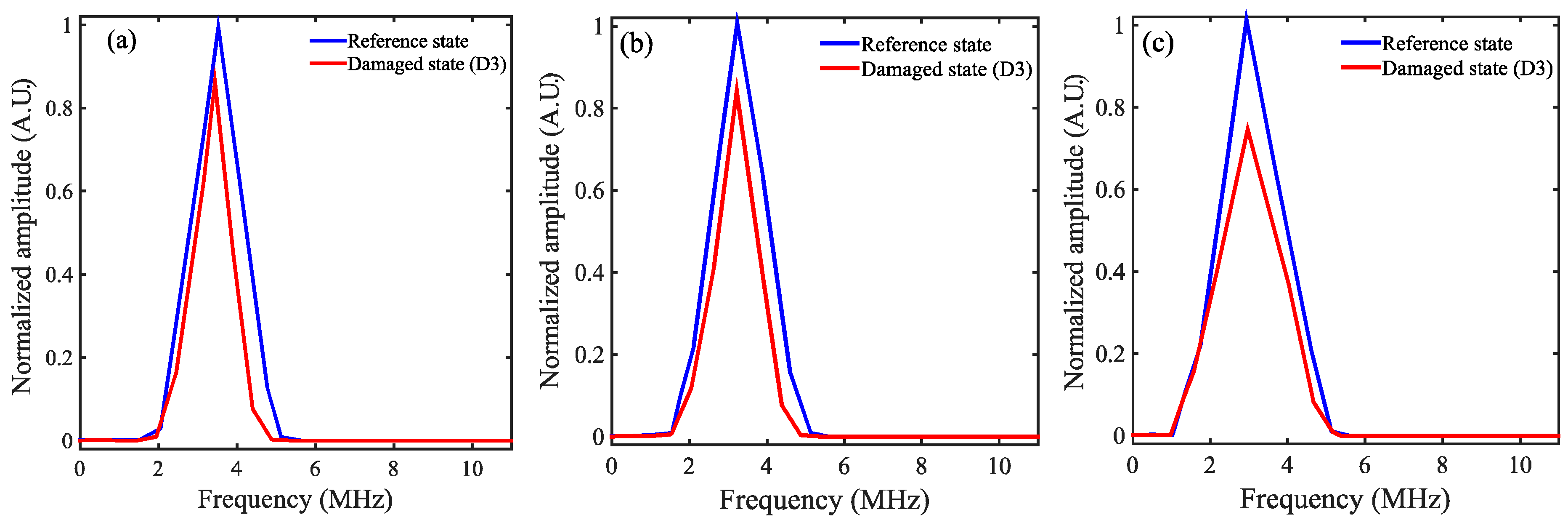
| Reference state | 3.58 MHz | 3.5 MHz | 3.46 MHz |
| Damaged state—3 | 3.45 MHz | 3.42 MHz | 3.4 MHz |
| % change in frequency | 3.63 | 2.2 | 1.77 |
| Damage Cases | Damage-1 | Damage-2 | Damage-3 |
|---|---|---|---|
| CI values | 0.391 | 0.405 | 0.587 |
| % change in CI | - | 3.5 | 50.12 |
© 2018 by the authors. Licensee MDPI, Basel, Switzerland. This article is an open access article distributed under the terms and conditions of the Creative Commons Attribution (CC BY) license (http://creativecommons.org/licenses/by/4.0/).
Share and Cite
Pamwani, L.; Habib, A.; Melandsø, F.; Ahluwalia, B.S.; Shelke, A. Single-Input and Multiple-Output Surface Acoustic Wave Sensing for Damage Quantification in Piezoelectric Sensors. Sensors 2018, 18, 2017. https://doi.org/10.3390/s18072017
Pamwani L, Habib A, Melandsø F, Ahluwalia BS, Shelke A. Single-Input and Multiple-Output Surface Acoustic Wave Sensing for Damage Quantification in Piezoelectric Sensors. Sensors. 2018; 18(7):2017. https://doi.org/10.3390/s18072017
Chicago/Turabian StylePamwani, Lavish, Anowarul Habib, Frank Melandsø, Balpreet Singh Ahluwalia, and Amit Shelke. 2018. "Single-Input and Multiple-Output Surface Acoustic Wave Sensing for Damage Quantification in Piezoelectric Sensors" Sensors 18, no. 7: 2017. https://doi.org/10.3390/s18072017
APA StylePamwani, L., Habib, A., Melandsø, F., Ahluwalia, B. S., & Shelke, A. (2018). Single-Input and Multiple-Output Surface Acoustic Wave Sensing for Damage Quantification in Piezoelectric Sensors. Sensors, 18(7), 2017. https://doi.org/10.3390/s18072017