1. Introduction
As a kind of angular momentum exchange actuator, control moment gyros (CMGs) have been widely used in spacecraft attitude control owing to their superior properties in simple structure, large torque, and high precision [
1,
2,
3,
4,
5]. A CMG typically consists of a high-speed rotor with large angular momentum and one or two low-speed gimbals [
6,
7]. According to torque instructions, the rotor can be rotated by gimbal motions driven by gimbal servo systems. With the variations of the direction of the rotor momentum, gyroscopic torque will be produced to control spacecraft attitude. In order to output high-precision torque to meet the need of spacecraft attitude control with high accuracy and stability, the control precision of gimbal servo systems should be high enough.
However, there exist many disturbances in the gimbal servo systems, such as friction, torque ripple, the disturbance torque induced by the rotor imbalance [
8,
9,
10], etc. All these disturbances can deteriorate the control performance of gimbal servo systems significantly, especially the dynamic imbalance disturbance. With the amplitude proportional to the square of the rotor angular velocity and the same frequency as the rotor [
8,
11,
12,
13,
14], it has been a great hindrance to the high-performance control of gimbal servo systems, since the high speed of the rotor will lead to severe disturbance with higher frequency and larger amplitude. Therefore, it is necessary to obtain the information regarding the rotor dynamic imbalance before designing the gimbal servo systems for CMGs.
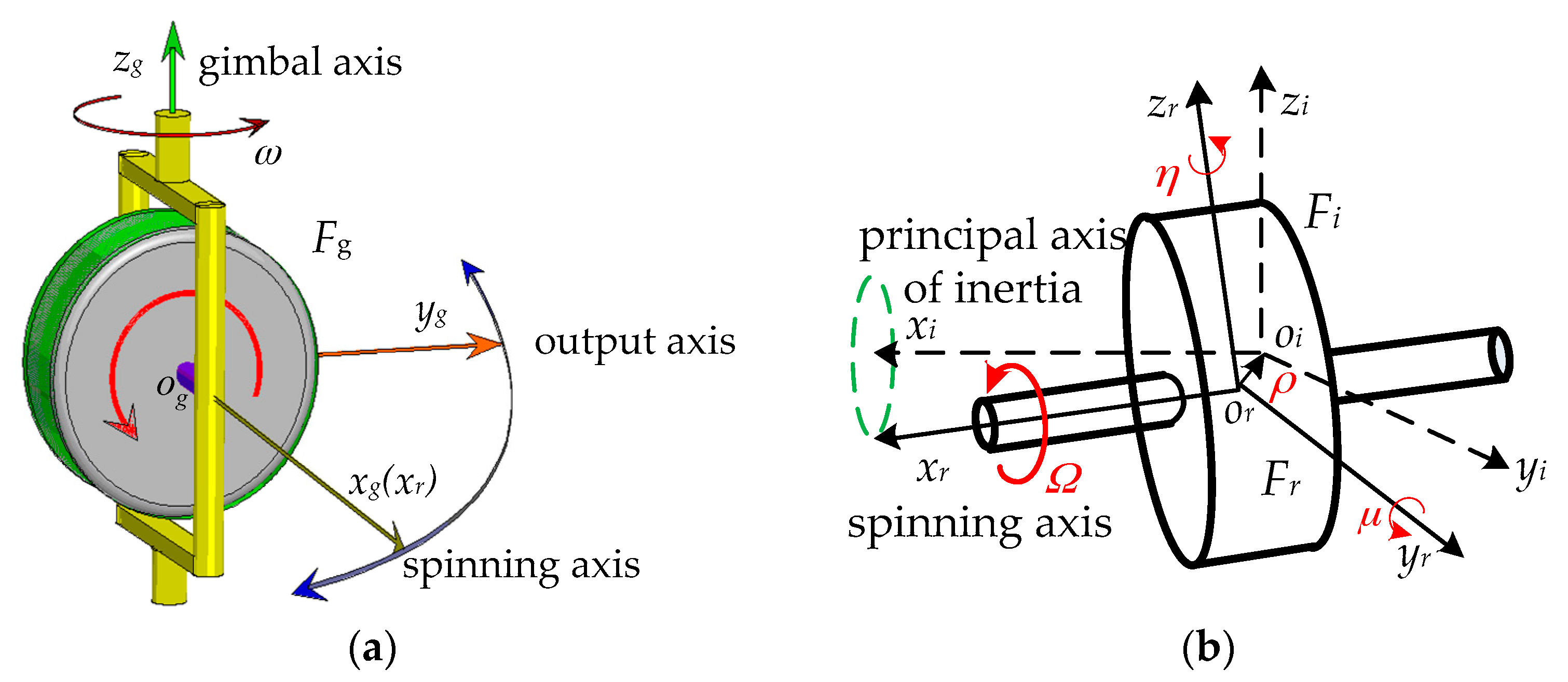
Rotor mass imbalance is caused by the asymmetry of the rotor with respect to the spinning axis, owing to nonuniform mass distribution and imperfections in manufacturing [
15,
16,
17]. Static imbalance results from the offset of the centroid from the spinning axis of the rotor. Dynamic imbalance results from the misalignment of the principal axis of inertia with respect to the spinning axis of the rotor. When the rotor rotates around the spinning axis, static and dynamic imbalance can produce radial centrifugal force and torque, respectively [
18,
19,
20]. Since only the torque can rotate the gimbal, the dominant factor affecting gimbal servo systems is the dynamic imbalance, not the static one.
For a free rotor, the dynamic imbalance can be measured by using well-developed methods and then reduced with correction devices by adding or subtracting correction masses [
21,
22]. Owing to the limits of practical devices, a certain residual imbalance still exists in the rotor after dynamic balancing [
23]. Furthermore, the dynamic imbalance may be changed by an error of assembly after the rotor is assembled on the mechanical bearing. In order to obtain the information of the dynamic imbalance for the assembled rotor, field dynamic balancing techniques can be used without disassembly [
24,
25]. However, these techniques are not suitable for the assembled CMGs owing to the effects of the gimbal motions.
For the measurement and suppression of the residual mass imbalance of magnetically suspended rotors installed in the equipment, various research results have been reported in literatures [
26]. In one study [
27], a disturbance observer was designed to estimate the matched disturbances, including imbalance, and then a composite control method was proposed to realize precision suspension of an active magnetic bearing (AMB) system. In another study [
28], a repetitive disturbance observer-based controller was developed specially to reject the disturbance caused by the rotor mass imbalance of an AMB system. Another study [
29] found that the lumped disturbances, including imbalance, were estimated by using disturbance equations and state measurements, and the vibrations were suppressed after disturbance compensation for electromagnetic actuators. However, these results are obtained by using the measurements of the rotor displacements which are only available in magnetically suspended rotors and not available in mechanical ones. Furthermore, the imbalance disturbance cannot be separated from the estimate of the total disturbance.
In order to obtain information about the dynamic imbalance for assembled rotors in CMGs, a gimbal disturbance observer is proposed in this paper. This observer is designed for a third-order system, describing dynamic imbalance disturbance and the other disturbances in the gimbal servo system. During the observer design, the total disturbance is regarded as a virtual measurement which can be achieved by using the inverse dynamics of the gimbal servo system. By using the gimbal disturbance observer, the dynamic imbalance disturbance can be separated from the total one, and the information of the rotor dynamic imbalance can be derived indirectly.
The rest of the paper is organized as follows. In
Section 2, mathematical models for rotor imbalance and gimbal servo systems in CMGs are introduced, and the problem of the paper is formulated. In
Section 3, the gimbal disturbance observer is designed for a third-order disturbance model, and the performance of the observer is analyzed by using the Lyapunov theory. In
Section 4, a semi-physical experiment is carried out to verify the effectiveness of the observer. Finally, conclusions are given in
Section 5.
3. Indirect Measurement of Rotor Dynamic Imbalance
In this section, a third-order model is first established to describe the characteristics of the rotor dynamic imbalance disturbance and the other disturbances. Then, a gimbal disturbance observer is designed for the third-order disturbance model to estimate the rotor dynamic imbalance disturbance along the gimbal axis. Gain tuning guidelines and observer performance are also discussed in this section.
3.1. Disturbance Model
Denote the total disturbance in Equation (4) by
d, i.e.,
d = Tdz +
Tm +
Tg +
Tu, then Equation (4) can be rewritten as
Theoretically, the information of the total disturbance
d can be obtained from Equation (6) if both angular velocity
ω and electromagnetic torque
Te are available. In practice, it is not feasible to obtain
d by using Equation (6) since the calculation of the differential
will amplify higher-frequency noise components in
ω. Even though the total disturbance
d can be achieved, it is still difficult to obtain the information of the rotor dynamic imbalance torque
Tdz. In order to separate
Tdz from
d, it is necessary to find characteristics that differentiate
Tdz from the other disturbances. From Equation (3), it is obvious that
Tdz is a sinusoidal function of time with a fixed angular frequency
Ω, and the second-order derivative of
Tdz can be written as
According to Equations (3) and (7), the following equation can be obtained as
Let
x1 =
Tdz,
x2 =
,
x3 =
Tm +
Tg +
Tu, then a third-order state-space model can be derived from Equation (8) to describe the disturbance dynamics, as follows:
where
δ(
t) denotes the varying rate of
x3.
Regard
d in Equation (6) as a virtual measurement of the total disturbance, then the virtual output equation of System (9) can be written as
Let
,
,
,
, then we can rewrite Equations (9) and (10) in a compact form as
Thus, the dynamics of the rotor dynamic imbalance disturbance and the other disturbances in the gimbal servo system can be described by Equation (11). According to Equation (11), the observation matrix can be expressed as
Since rank (Qc) = 3, the pair (A,C) is observable; thus, a gimbal disturbance observer can be designed to estimate the disturbances.
3.2. Gimbal Disturbance Observer Design
In order to obtain the information of the rotor dynamic imbalance disturbance along the gimbal axis, a gimbal disturbance observer will be designed for Equation (11).
Let
and
represent the estimate of
x and the prediction of
d, respectively. According to the theory of Luenberger observer design, a state observer for Equation (11) can be designed as
where
L is the observer gain matrix with dimensions of 3 × 1.
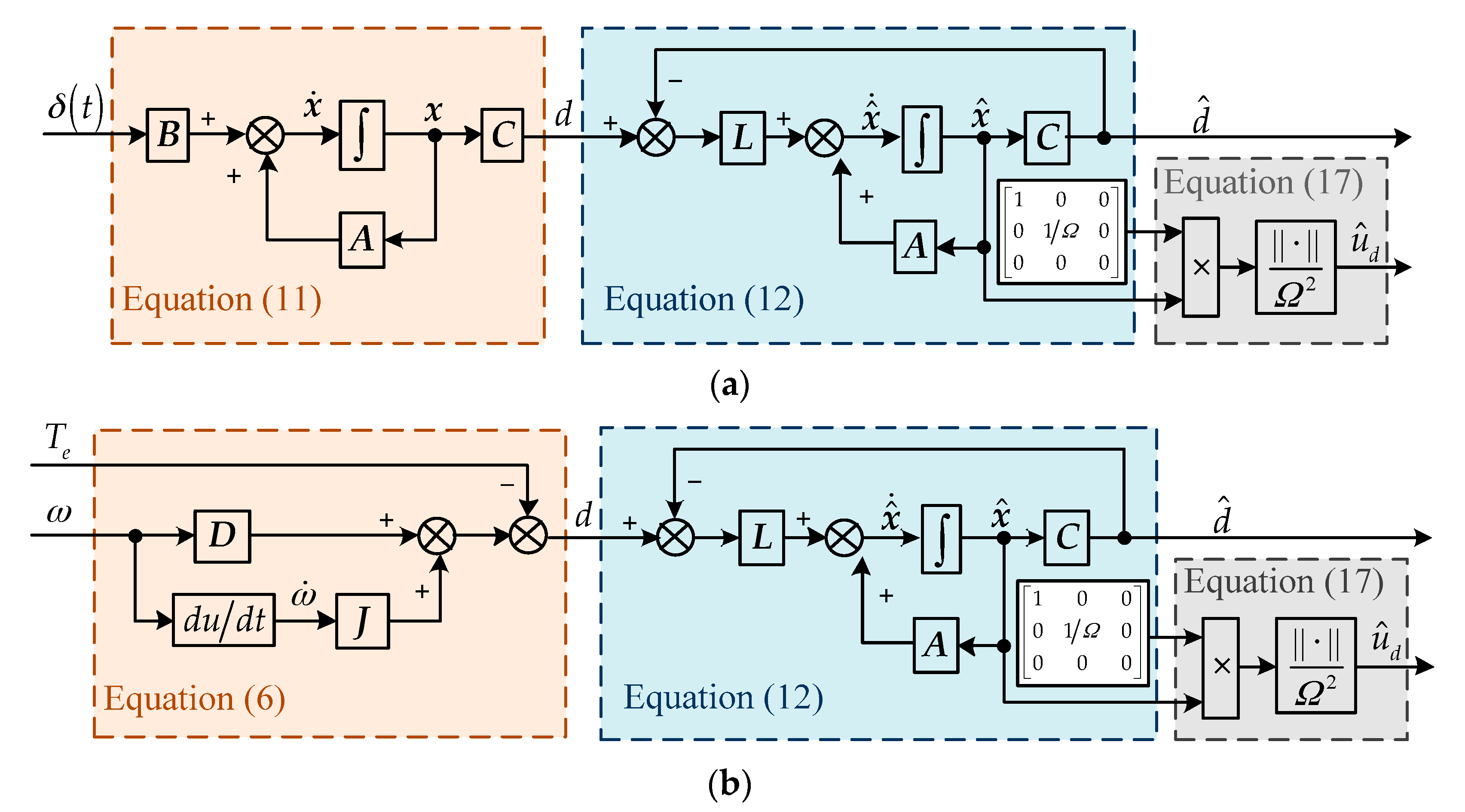
The relationship between Equation (11) and Equation (12) is shown in
Figure 2a. However, the output
d in the observer (12) is only a virtual measurement, and it cannot be measured directly. In this paper, the information of
d can be obtained indirectly from the system dynamics. According to the information of the angular velocity
ω and electromagnetic torque
Te,
d can be calculated from Equation (6). By substituting Equation (6) into Equation (12), the observer with indirect measurement of
d can be derived as
Then the observer with indirect measurement of
d can be plotted in
Figure 2b. Since
, Equation (13) can be rewritten as
In order to avoid the calculation of
in Equation (14), an auxiliary variable
z is introduced to satisfy
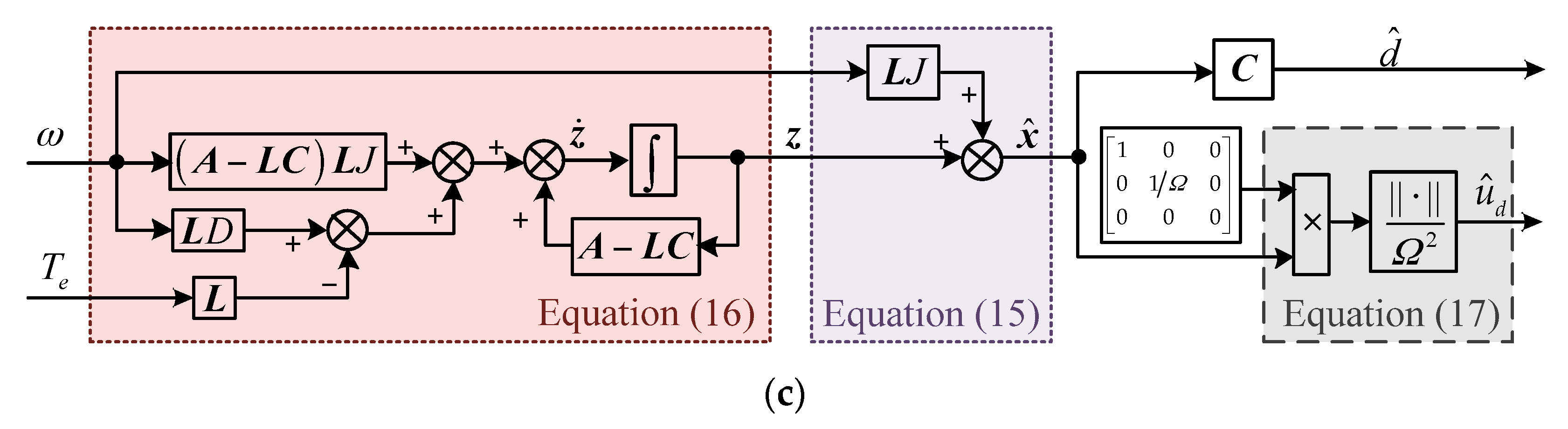
By using the auxiliary variable z in Equation (15), the angular acceleration can be eliminated in Equation (14), which can be changed into the following form as
Thus, the gimbal disturbance observer can be formulated by Equations (15) and (16), and it is shown in
Figure 2c. According to gimbal velocity
ω and electromagnetic torque
Te, the auxiliary variable
z can be derived from Equation (16) and the estimate
can be derived from Equation (15) in turn. According to the definition of state variables
x1 and
x2, the quantity of the rotor dynamic imbalance can be estimated as
.
3.3. Observer Convergence Analysis
In order to analyze the convergence of the gimbal disturbance observer in Equations (15) and (16), the error dynamics of the observer should be obtained first. Since the observer in Equations (15) and (16) is obtained by the variable substitution of Equation (12), the error dynamics for Equation (12) can be examined instead.
By defining the estimation errors as
and
, the error dynamics of the observer can be derived from Equations (11) and (12), as follows:
Since the pair (A, C) is observable, the matrix (A − LC) can be Hurwitz by choosing the suitable gain matrix L. Then, given any matrix Q > 0, there must exist a unique matrix P > 0 such that
For the error dynamics in Equation (18), choose the Lyapunov candidate function as
Taking the time derivative of Equation (20) along with Equations (18) and (19) gives
Let
λ1,
λ2, and
δm denote the minimal eigenvalue of
Q, the maximal eigenvalue of
P, and the upper bound of
δ(
t), respectively. Thus, Equation (21) can be enlarged as
where ‖·‖ denotes 2-norm of a vector or matrix.
When , we have which will drive the trajectory of into a bounded region . The upper bound of R depends on λ1, λ2, and δm, and it can be decreased by regulating the gain matrix L.
3.4. Gain Tuning Guidelines
According to Equation (18), the transfer function from
δ(
s) to the disturbance estimation error
can be obtained as
where
I is an identity matrix with dimensions of 3 × 3.
Let L = [l1, l2, l3]T, then G(s) in Equation (23) can be rewritten as
From Equation (24), it is known that the characteristic polynomial of the error system in Equation (18) is as follows:
If the bandwidth of Equation (18) is chosen as λ > 0, and the poles of Equation (24) are configured as −λ, −λ ± jΩ, then the characteristic polynomial can be written as
By comparing Equation (25) with Equation (26), the observer gains can be determined by
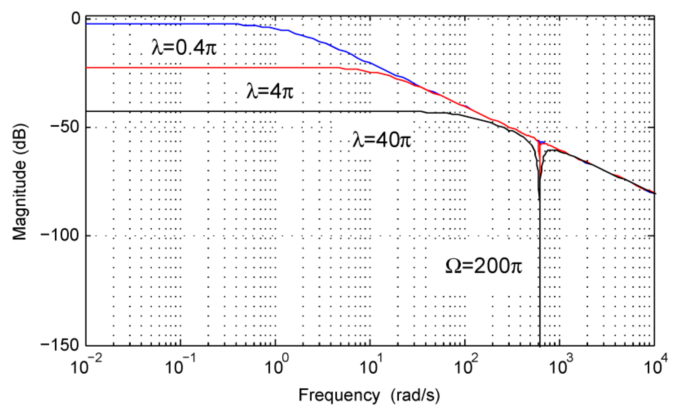
Thus, the problem of the observer gain tuning can be transformed into the choice of the bandwidth λ by using Equation (27). To demonstrate the effects of differences in bandwidth λ on the performance of the gimbal disturbance observer, the amplitude–frequency characteristics of G(s) can be used as an example.
By assuming the rotor velocity
Ω = 200
π rad/s, the amplitude-frequency characteristics of
G(
s) can be plotted in
Figure 3 for
λ = 0.4
π, 4
π, 40
π rad/s. From
Figure 3, it can be concluded that the disturbance
d can be estimated precisely, even though the bandwidth
λ is much less than the angular velocity
Ω of the rotor. It is worth noting that the effect of the model uncertainty
δ(
t) can be more strongly attenuated with the rise of the bandwidth. However, a higher bandwidth can amplify noise components in the measurements of gimbal velocity
ω and electromagnetic torque
Te. The choice of the bandwidth
λ is still a tradeoff between the attenuation ability of the model uncertainty and the measurement noise.
3.5. Discussions
According to the definition of L, the disturbance observer in Equation (12) can be rewritten as
Since , Equation (28) can be rewritten as
Under zero initial conditions, the Laplace transformation of Equation (29) can be derived as
According to Equation (30), the transfer functions from the total disturbance d to and can be obtained as follows.
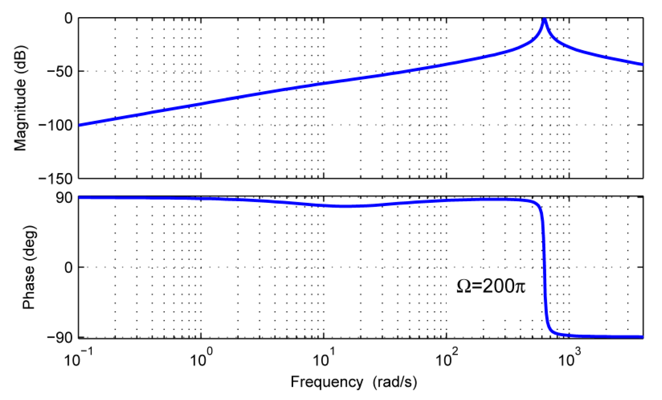
In order to analyze the estimation performance of
and
in the frequency domain, we can take the observer bandwidth
λ = 4
π rad/s as an example. According to Equation (27), the observer gains
l1,
l2, and
l3 will have definite values, and the frequency characteristics of
G1(
s) and
G3(
s) can be plotted in
Figure 4 and
Figure 5, respectively.
From
Figure 4, it is obvious that the amplitude is
and the phase is
for the rotor imbalance frequency
Ω. This means that the rotor dynamic imbalance disturbance in
d can be completely transmitted to
. While for the other components with the frequency much less or more than
Ω, the transmission gains to
are greatly reduced. Therefore,
can realize the estimation of the rotor dynamic imbalance disturbance and the effects of the other frequency contents in
d are very small.
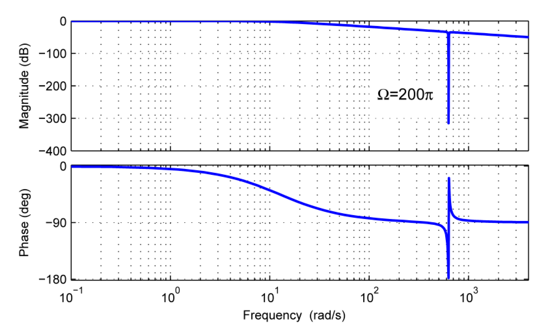
From
Figure 5, it can be seen that
G3(s) has the characteristics of a low-pass filter. When the frequency contents are much lower than the bandwidth of 4
π rad/s, they can be transmitted to
. When the frequency contents are much higher than the bandwidth, the transmission gains to
are greatly reduced. Especially for the rotor imbalance frequency, the amplitude
and the imbalance disturbance in
d cannot affect
.
From the analysis of
Figure 4 and
Figure 5, it can be concluded that the rotor dynamic imbalance and the other disturbances in
d can be estimated separately by using the gimbal disturbance observer. The rotor dynamic imbalance torque can be estimated by
, and the other disturbances can be estimated by
.
4. Experimental Results
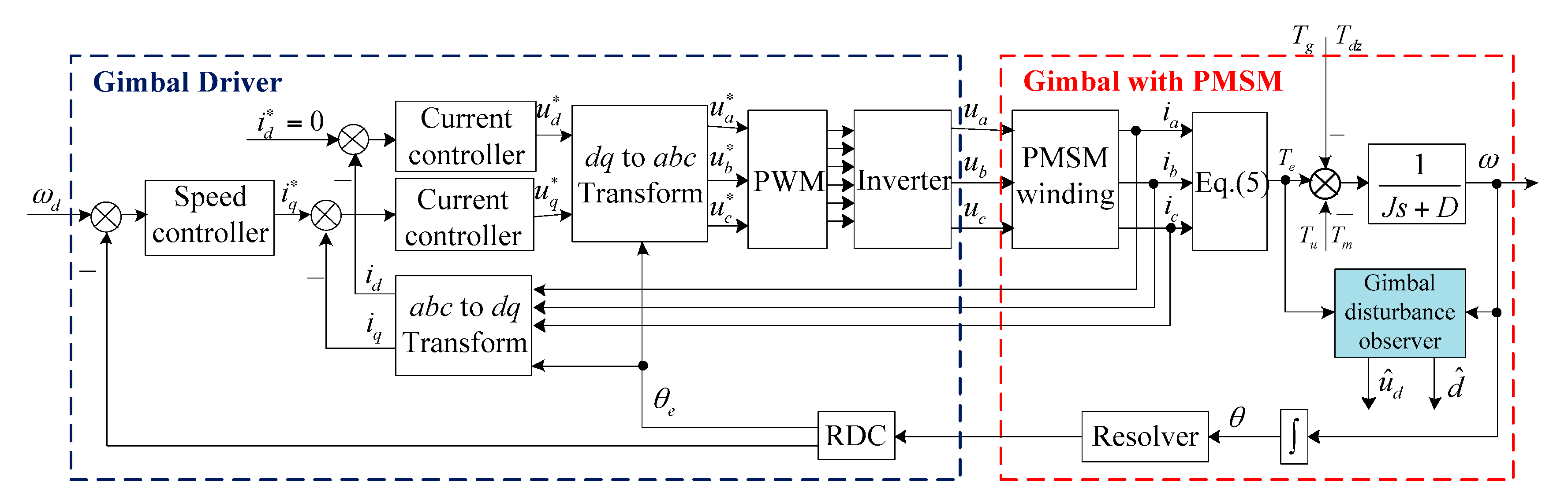
In order to verify the effectiveness of the gimbal disturbance observer, semi-physical experiments were carried out. The block diagram of the gimbal servo system and gimbal disturbance observer is shown in
Figure 6, and the details of the gimbal disturbance observer are shown in
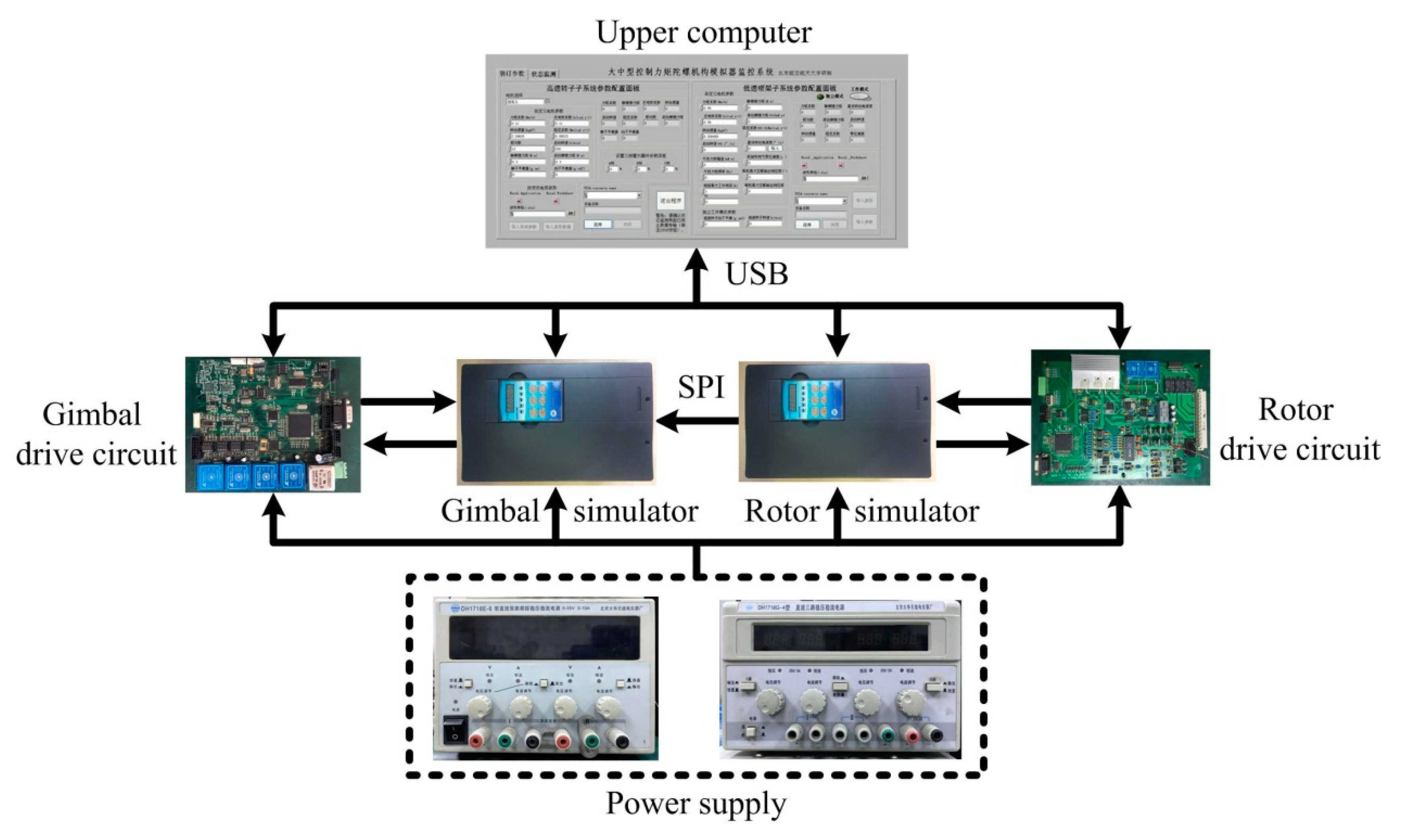
Figure 2c. The semi-physical experiment platform included a CMG simulator, CMG drive circuits, an upper computer, and power supplies, as shown in
Figure 7.
A CMG simulator is an electric load which has similar electrical and mechanical characteristics to practical CMG and has been used as a substitute for practical CMG to test CMG drive circuits in spacecraft engineering. It is composed of two parts, i.e., a gimbal simulator and a rotor simulator. The rotor simulator is in charge of simulating a brushless DC rotor motor with three switch-mode Hall position sensors, while the gimbal simulator is in charge of simulating a permanent magnet synchronous gimbal motor with two-channel resolvers. The rotor drive circuit is in charge of driving the rotor simulator, the information of which is transmitted to the gimbal simulator through serial peripheral interface (SPI). The gimbal drive circuit is in charge of driving the gimbal simulator, which can generate rotor dynamic imbalance torque and the other disturbances according to the rotor information and physical parameters. The physical parameters of the CMG simulator could be loaded by the upper computer, which also monitored the running states of the CMG simulator through USB. Since the actual value of the dynamic imbalance could be preset in the CMG simulator, it was very convenient to evaluate the performance of the indirect measurement method by comparing the estimated value with the preset one. When a practical CMG is used, the information of the actual value for the dynamic imbalance will be unavailable.
For the experiment, the preset parameters of the CMG simulator are listed in
Table 1. The gimbal simulator was controlled to run by the gimbal drive circuit at the desired velocity of 1°/s, while the rotor simulator was controlled to run by the rotor drive circuit at 3000 r/min, 6000 r/min, and 9000 r/min, respectively. In the gimbal drive circuit, the sampling rate of the gimbal velocity
ω and three-phase currents
ia,
ib, and
ic were 5kHz. According to Equation (5), the electromagnetic torque
Te can be derived from the sampled three-phase currents. By using the gimbal velocity
ω and electromagnetic torque
Te, the gimbal disturbance observer can be implemented with the bandwidth
λ = 4
π rad/s. Thus, the quantity of the rotor dynamic imbalance
ud can be estimated from Equation (18) by using the estimated states of the gimbal disturbance observer. The internal disturbance
Tm is mainly caused by unexpected factors in gimbal servo systems, such as current ripples, flux distortion, and bearing friction. Since the gimbal simulator was controlled to run by the gimbal drive circuit,
Tm had already existed in the system, so we did not need to set the parameter of
Tm additionally. The gyroscopic torque produced by spacecraft motion was set to −0.06 Nm. The unmodeled dynamic
Tu also already existed in the system.
By using the above parameters and the observer bandwidth, experimental results for three different rotor velocities could be achieved, as shown in
Figure 8,
Figure 9 and
Figure 10. Considering the transient process in the estimates of the quantity of the rotor dynamic imbalance, the mean of the estimates in the final 60 ms (i.e., from 0.94 s to 1 s) were taken as the final estimate. Additionally, the standard deviation (STD) was computed to evaluate the final estimate. Both the final estimate and the standard deviation are listed in
Table 2.
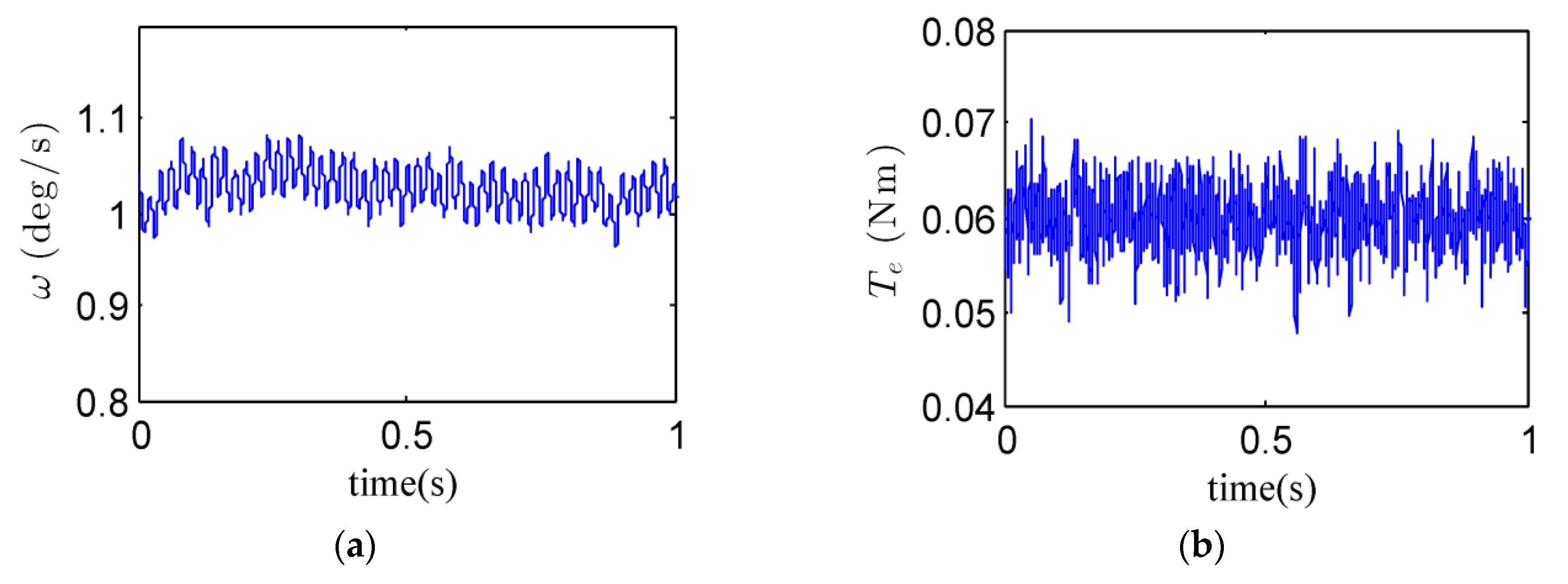
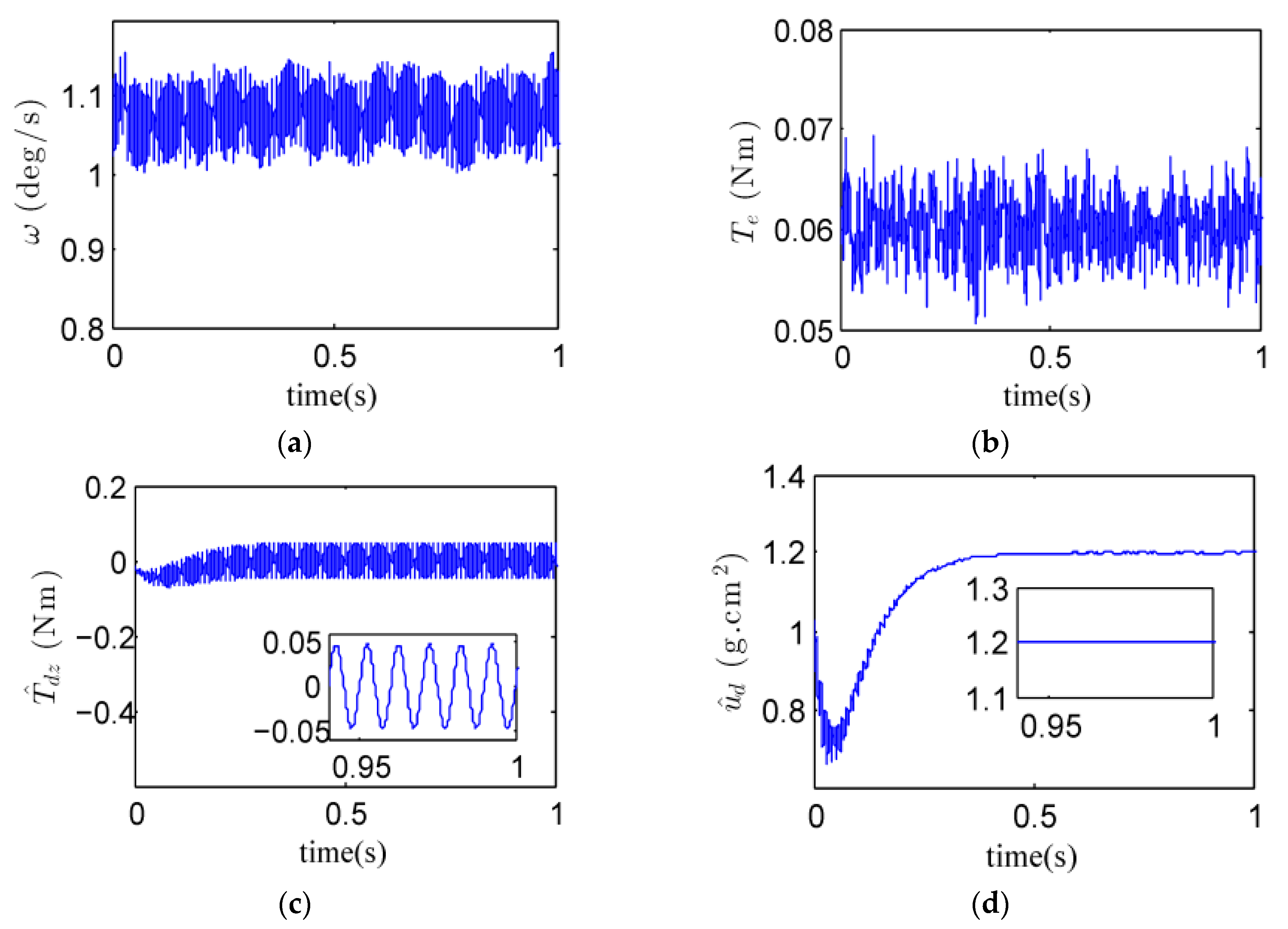
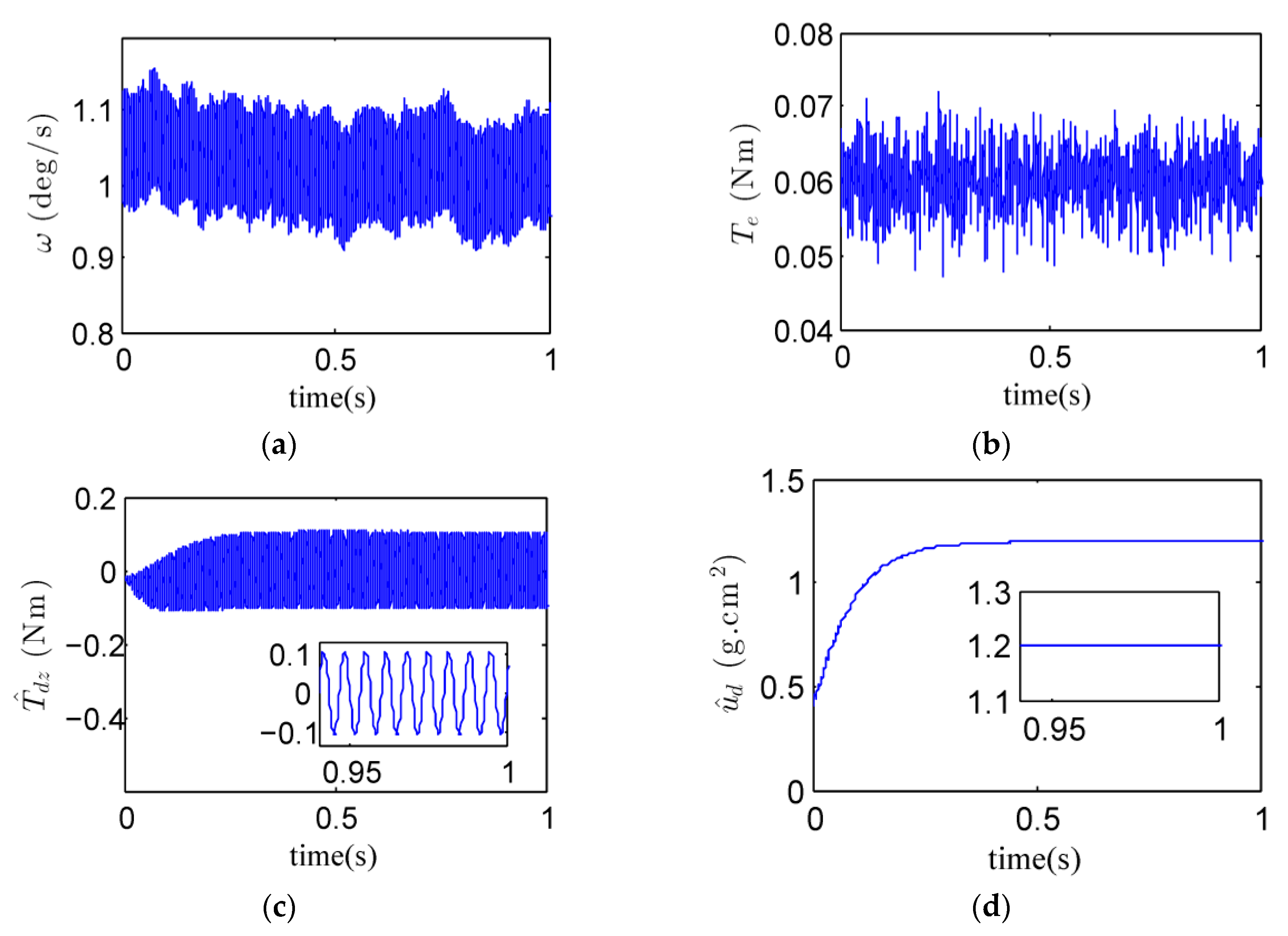
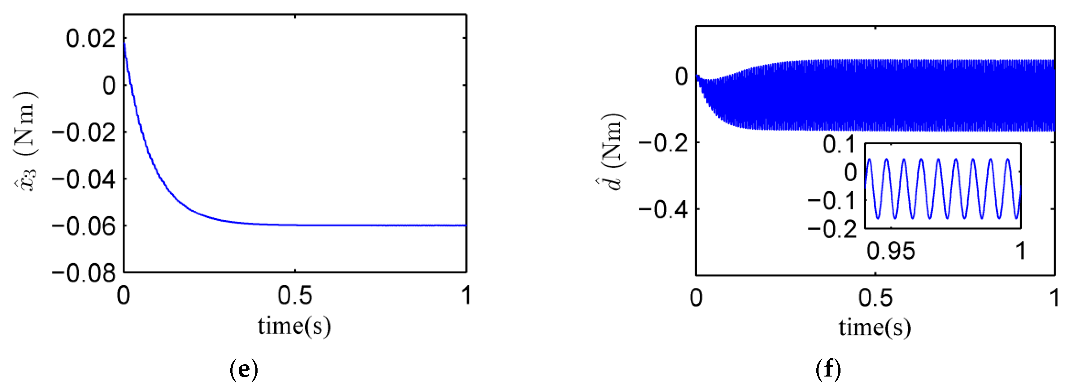
(1) For the rotor speed of 3000 r/min, the experimental curves and the estimate of the quantity of the rotor dynamic imbalance are shown in
Figure 8 and
Table 2, respectively. From
Figure 8a, it is obvious that the gimbal speed fluctuated periodically owing to the dynamic imbalance disturbance along the gimbal axis. From
Figure 8c, it is known that the amplitude of the dynamic imbalance torque exceeded 0.01 Nm. From
Figure 8d, it is known that the estimate of the quantity of the rotor dynamic imbalance is 1.1984 g·cm
2 with the standard deviation of 0.0023 g·cm
2.
Figure 8e shows the estimate of the other disturbances. Since the internal disturbance torque
Tm in the gimbal motor was quite small, the main component of
is the estimate of the gyroscopic torque
Tg produced by spacecraft motion, which was set to −0.06 Nm.
Figure 8f shows the estimate of the total disturbance
d. It can be concluded from
Figure 8c,e that the rotor dynamic imbalance and the other disturbances can be estimated separately by the proposed gimbal disturbance observer.
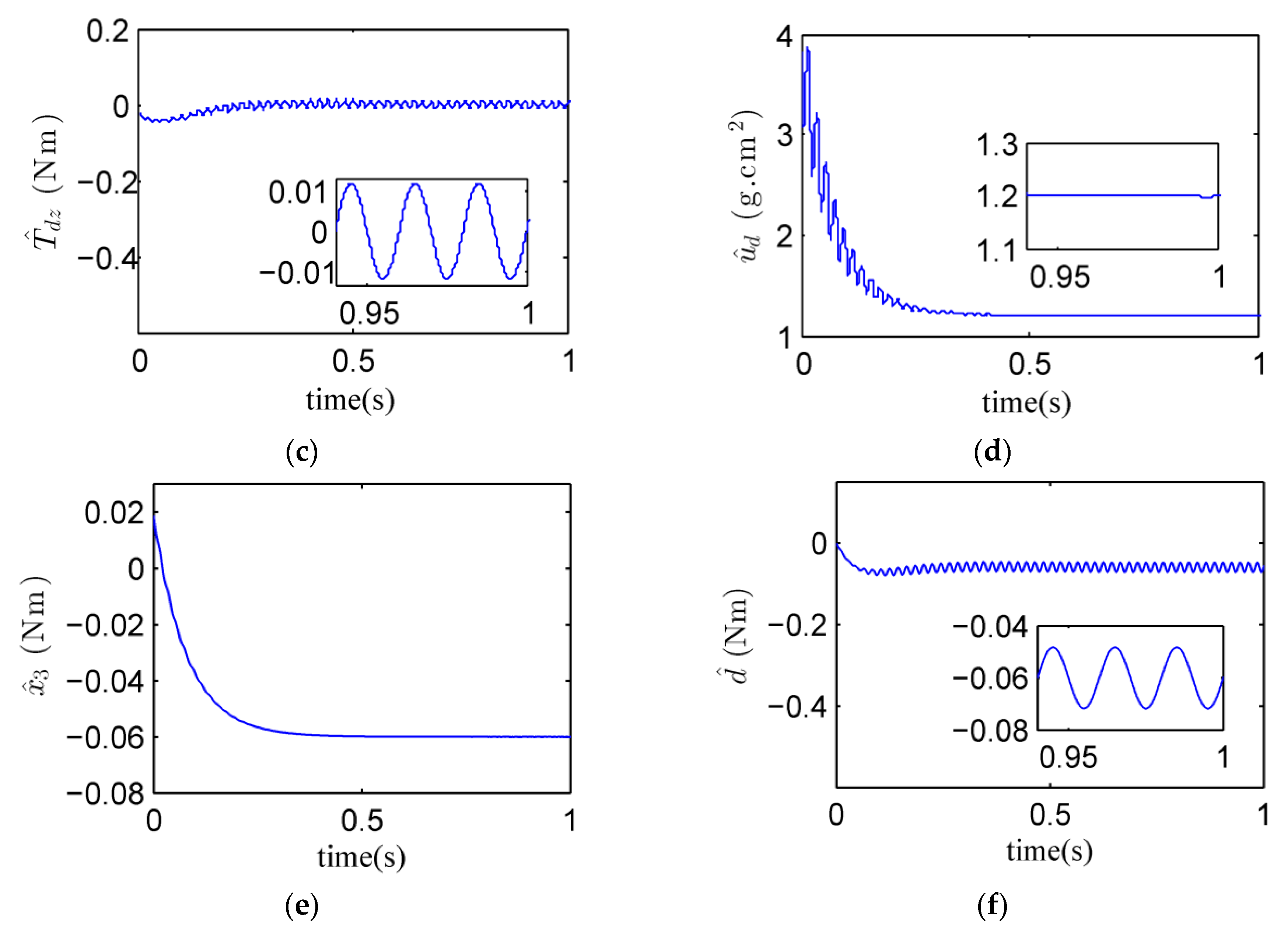
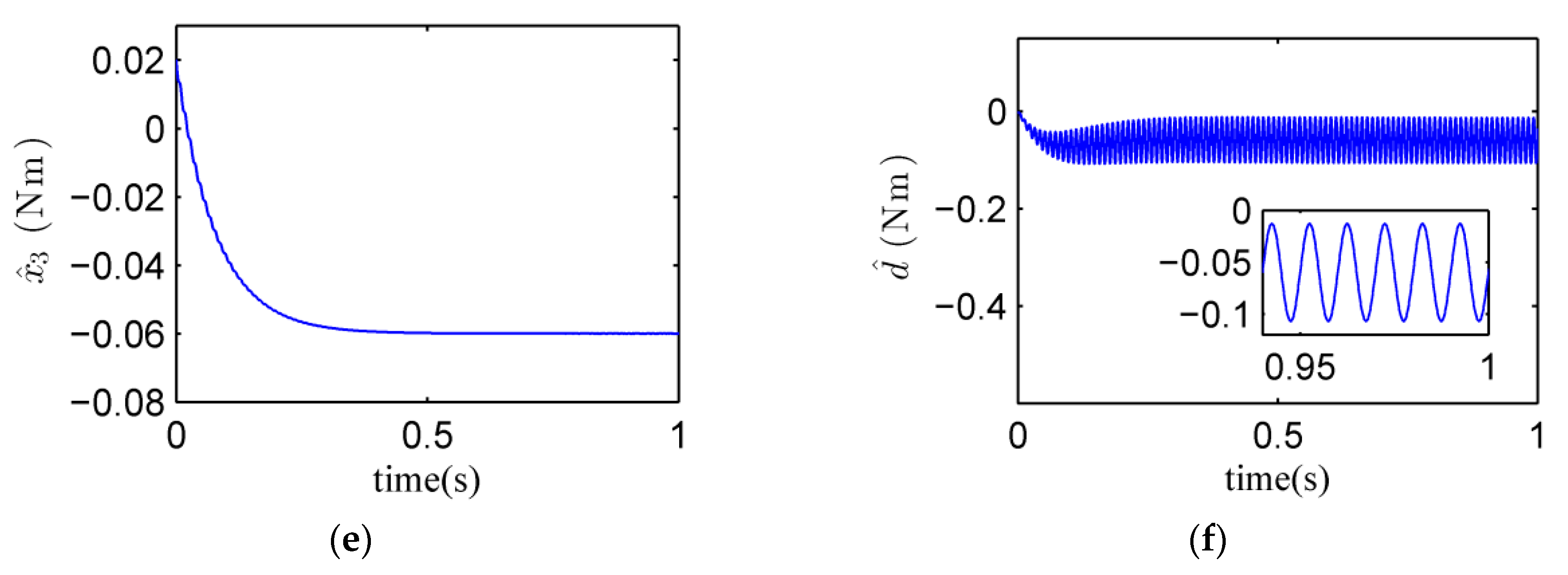
(2) For the rotor speed of 6000 r/min, the experimental curves and the estimate of the quantity of the rotor dynamic imbalance are shown in
Figure 9 and
Table 2, respectively. From
Figure 9a,c, it can be seen that the gimbal speed fluctuated with many more ripples, since the dynamic imbalance disturbance had a larger amplitude and frequency than that in
Figure 8. From
Table 2, it is known that the estimate of the quantity of the rotor dynamic imbalance is 1.2003 g·cm
2, and it is more accurate than the result derived from
Figure 8.
Figure 9e shows the estimate of the other disturbances
x3, which is approximately −0.06 Nm, and
Figure 9f shows the estimate of the total disturbance
d.
(3) For the rotor speed of 9000 r/min, the experimental curves and the estimate of the quantity of the rotor dynamic imbalance are shown in
Figure 10 and
Table 2, respectively. From
Figure 10a, it is clear that the fluctuations of the gimbal speed became heavier with the increase of the dynamic imbalance disturbance
Tdz in
Figure 10c. The estimate of the quantity of the rotor dynamic imbalance in
Table 2 is 1.1991 g·cm
2 with smaller standard deviation.
Figure 10e shows the estimate of the other disturbances
x3. Similar to the first two cases,
is also about −0.06 Nm.
Figure 10f shows the estimate of the total disturbance
d.
From the above results, it can be concluded that the rotor dynamic imbalance and the other disturbances could be estimated successfully and separately by the gimbal disturbance observer in all three experimental cases. Comparatively, the estimates of the latter two cases have higher precision than that of the first one since the sampled information became richer with the increase of the rotor speed at the fixed sampling frequency.


