An Efficient Neural-Network-Based Microseismic Monitoring Platform for Hydraulic Fracture on an Edge Computing Architecture


Abstract
1. Introduction
2. Related Work
3. Edge-to-Center LearnReduce Microseismic Monitoring Platform Design
3.1. Platform Structure
3.2. The Data Center in ELMMP
3.2.1. Overview of the Data Center Model
3.2.2. Training Set
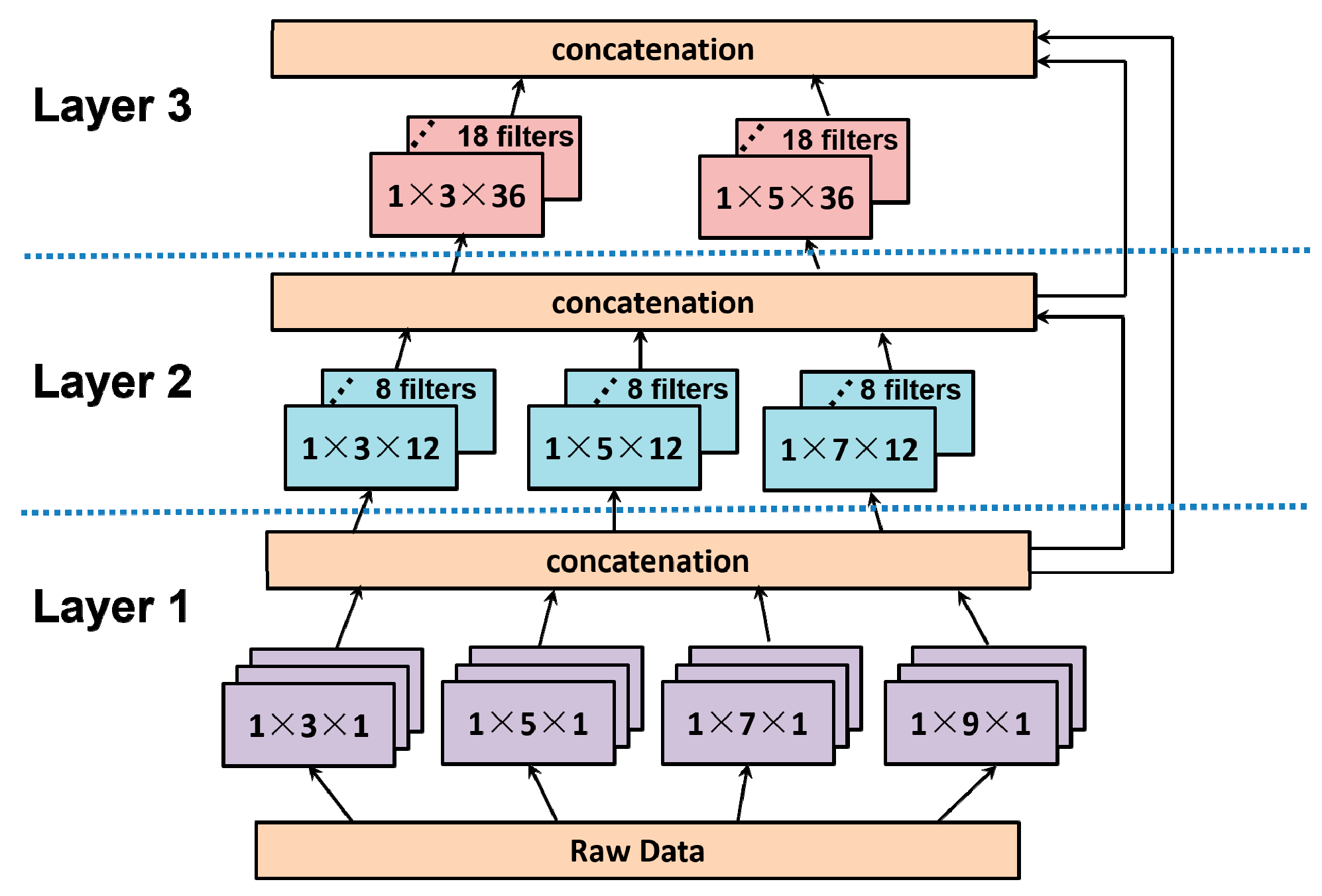
3.2.3. CNN Module
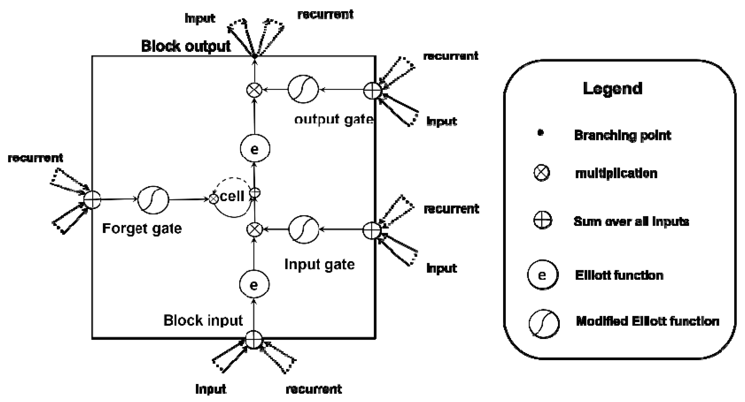
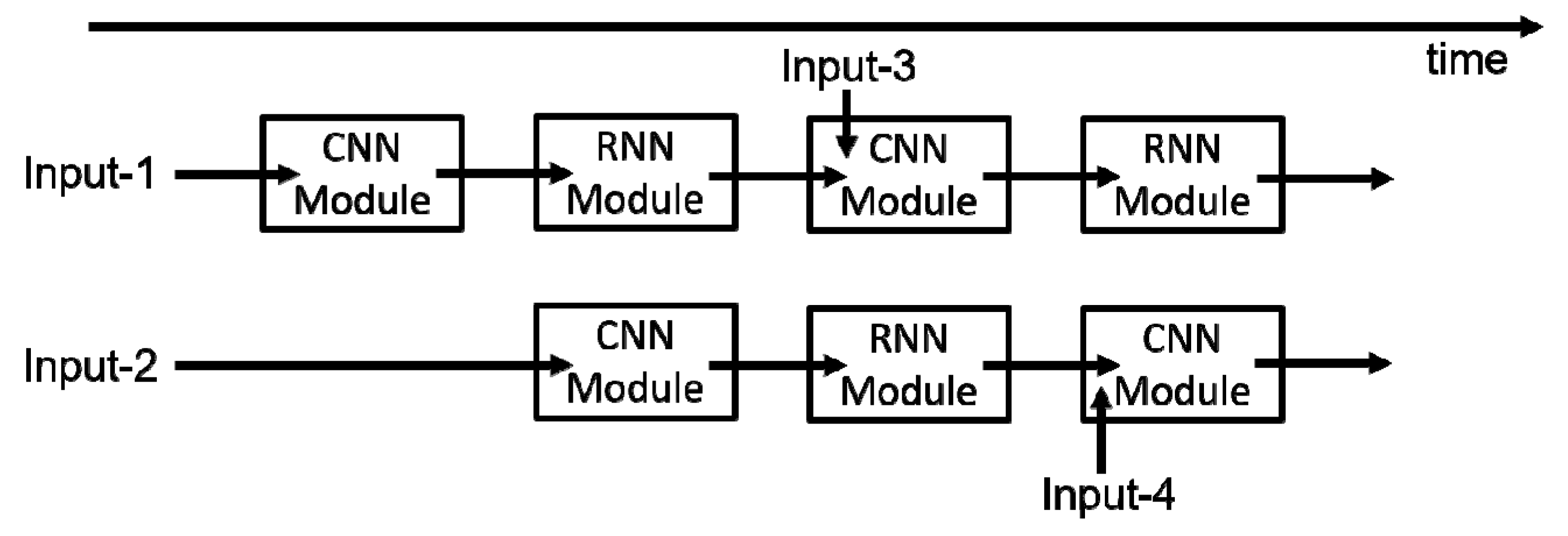
3.2.4. RNN Module
3.3. Edge Component in ELMMP
3.3.1. Overview of Edge Computing in ELMMP
3.3.2. Noise Reduction of Microseismic Data
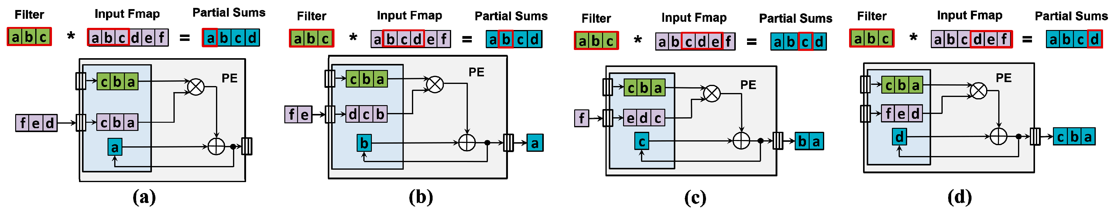
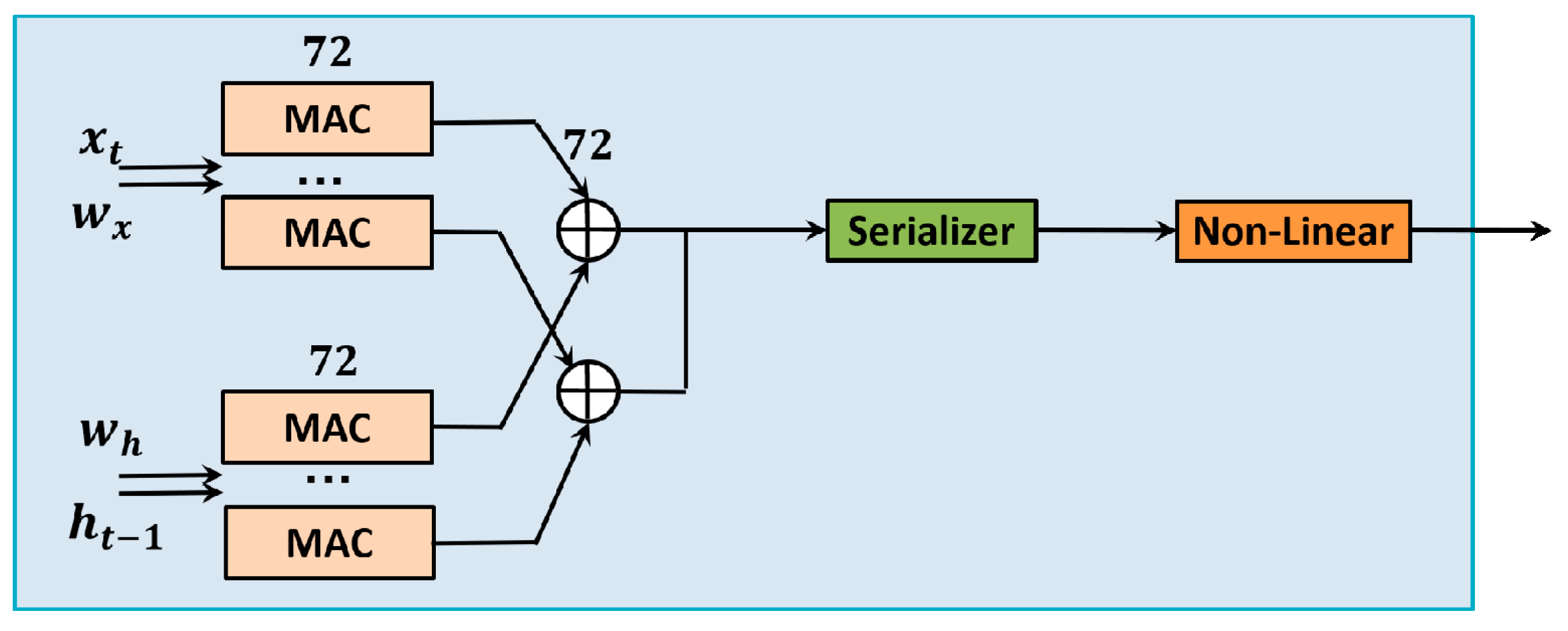
3.3.3. Implementation of the Neural Network
3.3.4. Probabilistic Inference Module
4. Evaluation
4.1. Simulation Results and Analysis
4.2. Measurement Results and Analysis
5. Conclusions
Author Contributions
Funding
Conflicts of Interest
References
- Maxwell, S. Microseismic hydraulic fracture imaging: The path toward optimizing shale gas production. Lead. Edge 2011, 30, 340–346. [Google Scholar] [CrossRef]
- Le Calvez, J.; Malpani, R.; Xu, J.; Stokes, J.; Williams, M. Hydraulic fracturing insights from microseismic monitoring. Oilfield Rev. 2016, 28, 16–33. [Google Scholar]
- Alexander, T.; Baihly, J.; Boyer, C.; Clark, B.; Waters, G.; Jochen, V.; Le Calvez, J.; Lewis, R.; Miller, C.K.; Thaeler, J.; et al. Shale gas revolution. Oilfield Rev. 2011, 23, 40–55. [Google Scholar]
- Huang, W.; Wang, R.; Li, H.; Chen, Y. Unveiling the signals from extremely noisy microseismic data for high-resolution hydraulic fracturing monitoring. Sci. Rep. 2017, 7, 11996. [Google Scholar] [CrossRef] [PubMed]
- Hydraulically Fractured Wells Provide Two-Thirds of U.S. Natural Gas Production. 2016. Available online: https://www.eia.gov/todayinenergy/detail.php?id=26112 (accessed on 5 June 2018).
- Hefley, W.E.; Wang, Y. Economics of Unconventional Shale Gas Development; Springer: Cham, Switzerland, 2016. [Google Scholar]
- Baig, A.; Urbancic, T. Microseismic moment tensors: A path to understanding FRAC growth. Lead. Edge 2010, 29, 320–324. [Google Scholar] [CrossRef]
- Martínez-Garzón, P.; Bohnhoff, M.; Kwiatek, G.; Zambrano-Narváez, G.; Chalaturnyk, R. Microseismic monitoring of CO2 injection at the Penn west enhanced oil recovery pilot project, Canada: Implications for detection of wellbore leakage. Sensors 2013, 13, 11522–11538. [Google Scholar] [CrossRef] [PubMed]
- Maxwell, S.C.; Urbancic, T.I. The role of passive microseismic monitoring in the instrumented oil field. Lead. Edge 2001, 20, 636–639. [Google Scholar] [CrossRef]
- Zhu, Y.; Li, N.; Sun, F.; Lin, J.; Chen, Z. Design and application of a borehole–surface microseismic monitoring system. Instrum. Sci. Technol. 2017, 45, 233–247. [Google Scholar] [CrossRef]
- Iqbal, N.; Al-Shuhail, A.A.; Kaka, S.I.; Liu, E.; Raj, A.G.; McClellan, J.H. Iterative interferometry-based method for picking microseismic events. J. Appl. Geophys. 2017, 140, 52–61. [Google Scholar] [CrossRef]
- Lee, M.; Byun, J.; Kim, D.; Choi, J.; Kim, M. Improved modified energy ratio method using a multi-window approach for accurate arrival picking. J. Appl. Geophys. 2017, 139, 117–130. [Google Scholar] [CrossRef]
- Akram, J.; Eaton, D.W. A review and appraisal of arrival-time picking methods for downhole microseismic data Arrival-time picking methods. Geophysics 2016, 81, KS71–KS91. [Google Scholar] [CrossRef]
- Zhu, D.; Li, Y.; Zhang, C. Automatic Time Picking for Microseismic Data Based on a Fuzzy C-Means Clustering Algorithm. IEEE Geosci. Remote Sens. Lett. 2016, 13, 1900–1904. [Google Scholar] [CrossRef]
- Chen, Y. Automatic microseismic event picking via unsupervised machine learning. Geophys. J. Int. 2017, 212, 88–102. [Google Scholar] [CrossRef]
- Hogarth, L.J.; Kolb, C.M.; Le Calvez, J.H. Controlled-source velocity calibration for real-time downhole microseismic monitoring. Lead. Edge 2017, 36, 172–178. [Google Scholar] [CrossRef]
- Li, Y.; Yang, T.H.; Liu, H.L.; Wang, H.; Hou, X.G.; Zhang, P.H.; Wang, P.T. Real-time microseismic monitoring and its characteristic analysis in working face with high-intensity mining. J. Appl. Geophys. 2016, 132, 152–163. [Google Scholar] [CrossRef]
- Wu, F.; Yan, Y.; Yin, C. Real-time microseismic monitoring technology for hydraulic fracturing in shale gas reservoirs: A case study from the southern Sichuan Basin. Nat. Gas Ind. B 2017, 4, 68–71. [Google Scholar] [CrossRef]
- Li, X.; Shang, X.; Wang, Z.; Dong, L.; Weng, L. Identifying P-phase arrivals with noise: An improved Kurtosis method based on DWT and STA/LTA. J. Appl. Geophys. 2016, 133, 50–61. [Google Scholar] [CrossRef]
- Mousavi, S.M.; Langston, C.A.; Horton, S.P. Automatic microseismic denoising and onset detection using the synchrosqueezed continuous wavelet transform. Geophysics 2016, 81, V341–V355. [Google Scholar] [CrossRef]
- Mousavi, S.M.; Langston, C.A. Adaptive noise estimation and suppression for improving microseismic event detection. J. Appl. Geophys. 2016, 132, 116–124. [Google Scholar] [CrossRef]
- Li, X.; Li, Z.; Wang, E.; Feng, J.; Chen, L.; Li, N.; Kong, X. Extraction of microseismic waveforms characteristics prior to rock burst using Hilbert–Huang transform. Measurement 2016, 91, 101–113. [Google Scholar] [CrossRef]
- Vera Rodriguez, I.; Bonar, D.; Sacchi, M. Microseismic data denoising using a 3C group sparsity constrained time-frequency transform. Geophysics 2012, 77, V21–V29. [Google Scholar] [CrossRef]
- Jia, R.S.; Sun, H.M.; Peng, Y.J.; Liang, Y.Q.; Lu, X.M. Automatic event detection in low SNR microseismic signals based on multi-scale permutation entropy and a support vector machine. J. Seismol. 2017, 21, 735–748. [Google Scholar] [CrossRef]
- Pugh, D.J.; White, R.S.; Christie, P.A. A Bayesian method for microseismic source inversion. Geophys. J. Int. 2016, 206, 1009–1038. [Google Scholar] [CrossRef]
- Vera Rodriguez, I.; Sacchi, M.D. Microseismic source imaging in a compressed domain. Geophys. J. Int. 2014, 198, 1186–1198. [Google Scholar] [CrossRef]
- Lin, J.; Zhang, X.; Wang, J.; Long, Y. The techniques and method for multi-hop seismic data acquisition based on compressed sensing. Chin. J. Geophs. 2017, 60, 4194–4203. [Google Scholar]
- Zhao, R.; Yan, R.; Wang, J.; Mao, K. Learning to monitor machine health with convolutional bi-directional LSTM networks. Sensors 2017, 17, 273. [Google Scholar] [CrossRef] [PubMed]
- He, Z.; Zhang, X.; Cao, Y.; Liu, Z.; Zhang, B.; Wang, X. LiteNet: Lightweight Neural Network for Detecting Arrhythmias at Resource-Constrained Mobile Devices. Sensors 2018, 18, 1229. [Google Scholar] [CrossRef] [PubMed]
- Ma, X.; Dai, Z.; He, Z.; Ma, J.; Wang, Y.; Wang, Y. Learning traffic as images: A deep convolutional neural network for large-scale transportation network speed prediction. Sensors 2017, 17, 818. [Google Scholar] [CrossRef] [PubMed]
- Mousavi, S.M.; Horton, S.P.; Langston, C.A.; Samei, B. Seismic features and automatic discrimination of deep and shallow induced-microearthquakes using neural network and logistic regression. Geophys. J. Int. 2016, 207, 29–46. [Google Scholar] [CrossRef]
- Gu, J.; Wang, Z.; Kuen, J.; Ma, L.; Shahroudy, A.; Shuai, B.; Liu, T.; Wang, X.; Wang, G.; Cai, J.; Chen, T. Recent advances in convolutional neural networks. Pattern Recognit. 2018, 77, 354–377. [Google Scholar] [CrossRef]
- Szegedy, C.; Vanhoucke, V.; Ioffe, S.; Shlens, J.; Wojna, Z. Rethinking the inception architecture for computer vision. In Proceedings of the IEEE Conference on Computer Vision and Pattern Recognition, Las Vegas, NV, USA, 27–30 June 2016; pp. 2818–2826. [Google Scholar]
- Lin, M.; Chen, Q.; Yan, S. Network in network. arXiv 2013, arXiv:1312.4400. [Google Scholar]
- Huang, G.; Liu, Z.; Weinberger, K.Q.; van der Maaten, L. Densely connected convolutional networks. In Proceedings of the IEEE Conference on Computer Vision and Pattern Recognition, Honolulu, HI, USA, 21–26 July 2017; Volume 1, p. 3. [Google Scholar]
- Hochreiter, S.; Schmidhuber, J. Long short-term memory. Neural Comput. 1997, 9, 1735–1780. [Google Scholar] [CrossRef] [PubMed]
- Greff, K.; Srivastava, R.K.; Koutník, J.; Steunebrink, B.R.; Schmidhuber, J. LSTM: A search space odyssey. IEEE Trans. Neural Netw. Learn. Syst. 2017, 28, 2222–2232. [Google Scholar] [CrossRef] [PubMed]
- Farzad, A.; Mashayekhi, H.; Hassanpour, H. A comparative performance analysis of different activation functions in LSTM networks for classification. Neural Comput. Appl. 2017, 1–5. [Google Scholar] [CrossRef]
- Han, S.; Kang, J.; Mao, H.; Hu, Y.; Li, X.; Li, Y.; Xie, D.; Luo, H.; Yao, S.; Wang, Y.; Yang, H. Ese: Efficient speech recognition engine with sparse LSTM on FPGA. In Proceedings of the 2017 ACM/SIGDA International Symposium on Field-Programmable Gate Arrays, Monterey, CA, USA, 22–24 February 2017; pp. 75–84. [Google Scholar]
- Yin, S.; Tang, S.; Lin, X.; Ouyang, P.; Tu, F.; Liu, L.; Wei, S. A high throughput acceleration for hybrid neural networks with efficient resource management on FPGA. IEEE Trans. Comput.-Aided Des. Integr. Circuits Syst. 2018. [Google Scholar] [CrossRef]
- Gao, N.; Zheng, F.; Wang, X.; Jiang, X.X.; Lin, J. High-speed download of seismographs using private cloud technology and a proportional integral derivative controller. Instrum. Sci. Technol. 2016, 44, 12–22. [Google Scholar] [CrossRef]


| SNR (dB) | STA/LTA Threshold | STA/LTA Accuracy (%) | STA/LTA Precision (%) | STA/LTA Recall (%) | Proposed Algorithm Accuracy (%) | Proposed Algorithm Precision (%) | Proposed Algorithm Recall (%) |
|---|---|---|---|---|---|---|---|
| 0 | 0.41 | 96.92 | 89.63 | 84.72 | 98.58 | 94.07 | 93.38 |
| −5 | 0.37 | 96.85 | 88.14 | 82.76 | 98.42 | 93.35 | 92.64 |
| −10 | 0.38 | 96.78 | 86.67 | 81.81 | 97.45 | 89.72 | 88.53 |
| −15 | 0.39 | 95.25 | 80.13 | 78.26 | 96.83 | 87.36 | 86.12 |
| SNR (dB) | Ratio of Data Reduced (%) |
|---|---|
| 0 | 89.17 |
| −5 | 89.67 |
| −10 | 90.67 |
| −15 | 88.75 |
© 2018 by the authors. Licensee MDPI, Basel, Switzerland. This article is an open access article distributed under the terms and conditions of the Creative Commons Attribution (CC BY) license (http://creativecommons.org/licenses/by/4.0/).
Share and Cite
Zhang, X.; Lin, J.; Chen, Z.; Sun, F.; Zhu, X.; Fang, G. An Efficient Neural-Network-Based Microseismic Monitoring Platform for Hydraulic Fracture on an Edge Computing Architecture. Sensors 2018, 18, 1828. https://doi.org/10.3390/s18061828
Zhang X, Lin J, Chen Z, Sun F, Zhu X, Fang G. An Efficient Neural-Network-Based Microseismic Monitoring Platform for Hydraulic Fracture on an Edge Computing Architecture. Sensors. 2018; 18(6):1828. https://doi.org/10.3390/s18061828
Chicago/Turabian StyleZhang, Xiaopu, Jun Lin, Zubin Chen, Feng Sun, Xi Zhu, and Gengfa Fang. 2018. "An Efficient Neural-Network-Based Microseismic Monitoring Platform for Hydraulic Fracture on an Edge Computing Architecture" Sensors 18, no. 6: 1828. https://doi.org/10.3390/s18061828
APA StyleZhang, X., Lin, J., Chen, Z., Sun, F., Zhu, X., & Fang, G. (2018). An Efficient Neural-Network-Based Microseismic Monitoring Platform for Hydraulic Fracture on an Edge Computing Architecture. Sensors, 18(6), 1828. https://doi.org/10.3390/s18061828