DE-Sync: A Doppler-Enhanced Time Synchronization for Mobile Underwater Sensor Networks


Abstract
1. Introduction
2. Related Work
3. Protocol Description
3.1. Overview of the DE-Sync
3.2. Impact of the Clock Skew
3.3. Details of the DE-Sync
3.4. Error Analysis
4. Performance Evaluation
4.1. Simulation Setup
4.2. Simulation Results and Analysis
4.2.1. Number of Calibration
4.2.2. Initial Skew
4.2.3. Response Time
4.2.4. Extent of Mobility
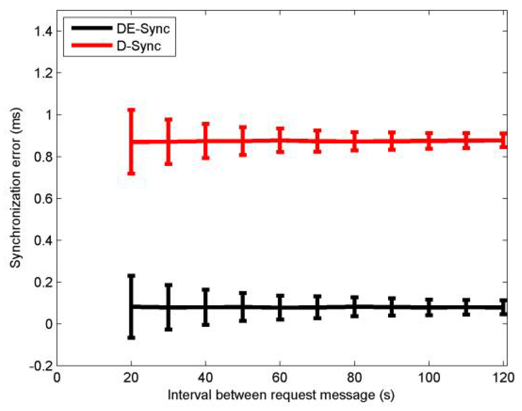
4.2.5. Internal between Request Messages
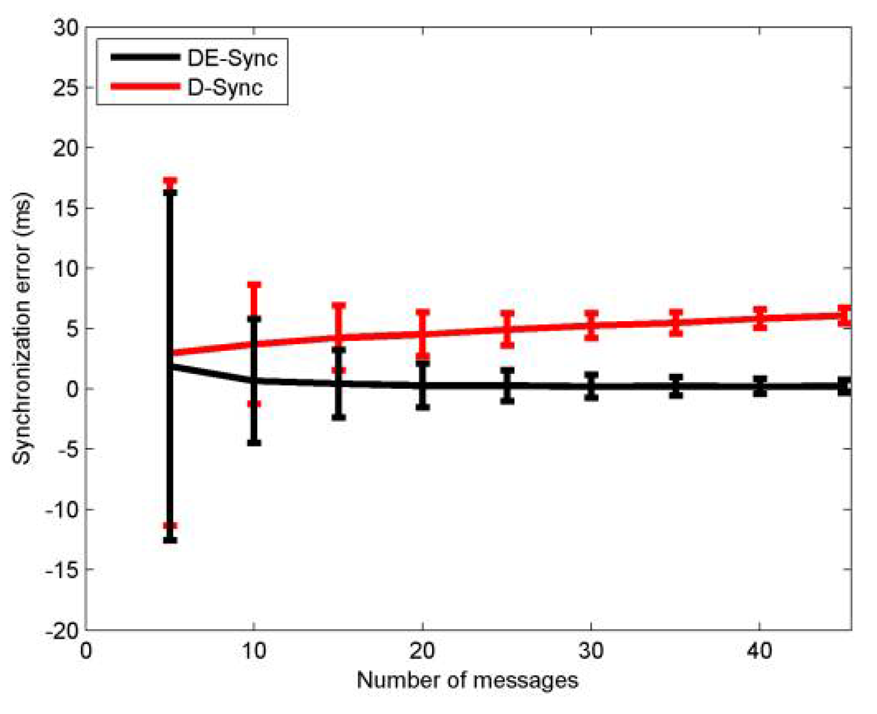
4.2.6. Number of Request Messages
4.2.7. Error After Synchronization
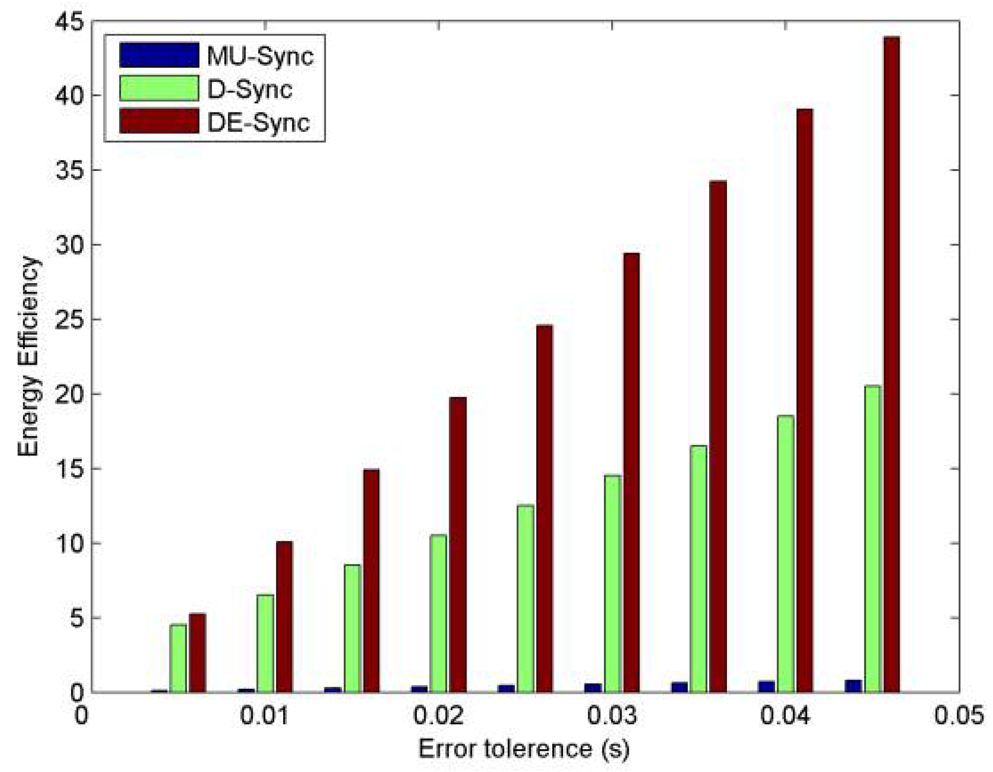
4.2.8. Comparison of Energy Efficiency
5. Conclusions and Future Work
Author Contributions
Funding
Conflicts of Interest
References
- Akyildiz, I.F.; Pompili, D.; Melodia, T. Underwater acoustic sensor networks: Research challenges. Ad Hoc Netw. 2005, 3, 257–279. [Google Scholar] [CrossRef]
- Heidemann, J.; Ye, W.; Wills, J.; Syed, A.; Li, Y. Research challenges and applications for underwater sensor networking. In Proceedings of the IEEE Wireless Communications and Networking Conference, Las Vegas, NV, USA, 3–6 April 2006; pp. 228–235. [Google Scholar] [CrossRef]
- Sivrikaya, F.; Yener, B. Time synchronization in sensor networks: A survey. Netw. IEEE 2004, 18, 45–50. [Google Scholar] [CrossRef]
- Elson, J.; Girod, L.; Estrin, D. Fine-grained network time synchronization using reference broadcasts. In Proceedings of the 5th Symposium on Operating Systems Design and Implementation, Boston, MA, USA, 9–11 December 2002; pp. 147–163. [Google Scholar] [CrossRef]
- Ganeriwal, S.; Ram, K.; Mani, B.S. Timing-sync protocol for sensor networks. In Proceedings of the 1st International Conference on Embedded Networked Sensor Systems, Los Angeles, CA, USA, 5–7 November 2003; pp. 138–149. [Google Scholar] [CrossRef]
- Maroti, M.; Kusy, B.; Simon, G.; Ledeczi, A. The flooding time synchronization protocol. In Proceedings of the 2nd International Conference on Embedded Networked Sensor Systems, Baltimore, MD, USA, 3–5 November 2004; pp. 39–49. [Google Scholar] [CrossRef]
- Cho, H.; Kim, J.; Baek, Y. Enhanced precision time synchronization for wireless sensor networks. Sensors 2011, 11, 7625–7643. [Google Scholar] [CrossRef] [PubMed]
- Shi, F.; Tuo, X.; Yang, S.X.; Li, H.; Shi, R. Multiple two-way time message exchange (ttme) time synchronization for bridge monitoring wireless sensor networks. Sensors 2017, 17, 1027. [Google Scholar] [CrossRef] [PubMed]
- Tavares Bruscato, L.; Heimfarth, T.; Pignaton de Freitas, E. Enhancing time synchronization support in wireless sensor networks. Sensors 2017, 17, 2956. [Google Scholar] [CrossRef] [PubMed]
- Wang, Z.; Zeng, P.; Zhou, M.; Li, D.; Wang, J. Cluster-based maximum consensus time synchronization for industrial wireless sensor networks. Sensors 2017, 17, 141. [Google Scholar] [CrossRef] [PubMed]
- Yoon, S.; Azad, A.K.; Oh, H.; Kim, S. Aurp: An auv-aided underwater routing protocol for underwater acoustic sensor networks. Sensors 2012, 12, 1827–1845. [Google Scholar] [CrossRef] [PubMed]
- Khan, J.U.; Cho, H.S. A distributed data-gathering protocol using auv in underwater sensor networks. Sensors 2015, 15, 19331–19350. [Google Scholar] [CrossRef] [PubMed]
- Wan, L.; Wang, Z.; Zhou, S.; Yang, T.C.; Shi, Z. Performance comparison of doppler scale estimation methods for underwater acoustic ofdm. J. Electr. Comput. Eng. 2012, 2012. [Google Scholar] [CrossRef]
- Sharif, B.S.; Neasham, J.; Hinton, O.R.; Adams, A.E. A computationally efficient doppler compensation system for underwater acoustic communications. IEEE J. Ocean. Eng. 2000, 25, 52–61. [Google Scholar] [CrossRef]
- Yang, T.C. Correlation-based decision-feedback equalizer for underwater acoustic communications. IEEE J. Ocean. Eng. 2005, 30, 865–880. [Google Scholar] [CrossRef]
- Li, B.; Zhou, S.; Stojanovic, M.; Freitag, L. Non-uniform doppler compensation for zero-padded ofdm over fast-varying underwater acoustic channels. In Proceedings of the Oceans, Aberdeen, UK, 18–21 June 2007; pp. 1–6. [Google Scholar] [CrossRef]
- Li, B.; Zhou, S.; Stojanovic, M.; Freitag, L.; Willett, P. Multicarrier communication over underwater acoustic channels with nonuniform doppler shifts. IEEE J. Ocean. Eng. 2008, 33, 198–209. [Google Scholar] [CrossRef]
- Johnson, M.; Freitag, L.; Stojanovic, M. Improved doppler tracking and correction for underwater acoustic communications. In Proceedings of the IEEE International Conference on Acoustics, Speech, and Signal Processing, Munich, Germany, 21–24 April 1997; p. 575. [Google Scholar] [CrossRef]
- Yu, L.; White, L.B. Optimum receiver design for broadband doppler compensation in multipath/doppler channels with rational orthogonal wavelet signaling. IEEE Trans. Signal Process. 2007, 55, 4091–4103. [Google Scholar] [CrossRef]
- Mason, S.; Berger, C.; Zhou, S.; Willett, P. Detection, synchronization, and doppler scale estimation with multicarrier waveforms in underwater acoustic communication. IEEE J. Sel. Areas Commun. 2008, 26, 1638–1649. [Google Scholar] [CrossRef]
- Salberg, A.B.; Swami, A. Doppler and frequency-offset synchronization in wideband OFDM. IEEE Trans. Wirel. Commun. 2005, 4, 2870–2881. [Google Scholar] [CrossRef]
- Ma, L.; Qiao, G.; Liu, S. A combined doppler scale estimation scheme for underwater acoustic OFDM system. J. Comput. Acoust. 2015, 23, 1540004. [Google Scholar] [CrossRef]
- Liu, S.; Lu, M.; Hui, L.; Chen, T.; Gang, Q. Design and implementation of OFDM underwater acoustic communication algorithm based on omap-l138. In Proceedings of the International Conference on Underwater Networks & Systems, Rome, Italy, 12–14 November 2014; p. 12. [Google Scholar] [CrossRef]
- Ma, L.; Qiao, G.; Liu, S. Heu OFDM-modem for underwater acoustic communication and networking. In Proceedings of the International Conference on Underwater Networks & Systems, Rome, Italy, 12–14 November 2014; p. 14. [Google Scholar] [CrossRef]
- Syed, A.A.; Heidemann, J. Time synchronization for high latency acoustic networks. In Proceedings of the 25th IEEE International Conference on Computer Communications, Barcelona, Spain, 23–29 April 2006; pp. 1–12. [Google Scholar] [CrossRef]
- Chirdchoo, N.; Soh, W.S.; Chua, K.C. Mu-sync: A time synchronization protocol for underwater mobile networks. In Proceedings of the Third ACM International Workshop on Underwater Networks, San Francisco, CA, USA, 15 September 2008; pp. 35–42. [Google Scholar] [CrossRef]
- Liu, J.; Zhou, Z.; Peng, Z.; Cui, J.H. Mobi-sync: Efficient time synchronization for mobile underwater sensor networks. In Proceedings of the Global Telecommunications Conference, Miami, FL, USA, 6–10 December 2010; pp. 1–5. [Google Scholar] [CrossRef]
- Lu, F.; Mirza, D.; Schurgers, C. D-sync: Doppler-based time synchronization for mobile underwater sensor networks. In Proceedings of the Fifth ACM International Workshop on UnderWater Networks, Woods Hole, MA, USA, 30 September–1 October 2010; pp. 1–8. [Google Scholar] [CrossRef]
- Liu, J.; Wang, Z.; Peng, Z.; Zuba, M. Tsmu: A time synchronization scheme for mobile underwater sensor networks. In Proceedings of the IEEE Global Telecommunications Conference, Kathmandu, Nepal, 5–9 December 2011; pp. 1–6. [Google Scholar] [CrossRef]
- Xie, P.; Zhou, Z.; Peng, Z.; Cui, J.H.; Shi, Z. Sdrt: A reliable data transport protocol for underwater sensor networks. Ad Hoc Netw. 2010, 8, 708–722. [Google Scholar] [CrossRef]
- Pallares, O.; Bouvet, P.J.; Rio, J.D. Ts-muwsn: Time synchronization for mobile underwater sensor networks. IEEE J. Ocean. Eng. 2016, 41, 763–775. [Google Scholar] [CrossRef]
- Liu, J.; Wang, Z.; Cui, J.-H.; Zhou, S.; Yang, B. A joint time synchronization and localization design for mobile underwater sensor networks. IEEE Trans. Mob. Comput. 2016, 15, 530–543. [Google Scholar] [CrossRef]


| Parameters | Description |
|---|---|
| A | Beacon node |
| B | Unsynchronized node |
| α | Clock skew |
| β | Clock offset |
| am | Doppler scale factor induced by the node mobility |
| vm | Average relative speed of nodes |
| c | Sound propagation speed |
| aAB | Measured Doppler scaling factor from A to B |
| aBA | Measured Doppler scaling factor from B to A |
| vAB | Measured relative speed from A to B |
| vBA | Measured relative speed from B to A |
| T1 | Sending time-stamp of unsynchronized node |
| T4 | Receiving time-stamp of unsynchronized node |
| T2 | Receiving time-stamp of beacon |
| T3 | Sending time-stamp of beacon |
| t2, t3 | Reference time at T2 and T3 |
| t1, t4 | Reference time at T1 and T4 |
| Tbackoff | Response time, that is T3 − T2 |
| τ1 | Propagation delay of synchronization request from B to A |
| τ2 | Propagation delay of synchronization response from A to B |
| Δd | Relative moving distance from t2 to t4 |
| Parameters | Value |
|---|---|
| Max distance (dmax) | 1000 m |
| Maximum relative speed (vmax) | 5 m/s |
| Maximum relative acceleration (Amax) | 0.1 m/s2 |
| Maximum clock skew (αmax) | 0.1 × 10⁶ ppm |
| Clock offset (β) | 80 ppm |
| Response time (Tbackoff) | 1 s |
| Interval between request messages (Minterval) | 3 s |
| Number of messages (N) | 25 |
| Clock granularity (Tgra) | 1 µs |
| Reception jitter (Tjitter) | 15 µs |
© 2018 by the authors. Licensee MDPI, Basel, Switzerland. This article is an open access article distributed under the terms and conditions of the Creative Commons Attribution (CC BY) license (http://creativecommons.org/licenses/by/4.0/).
Share and Cite
Zhou, F.; Wang, Q.; Nie, D.; Qiao, G. DE-Sync: A Doppler-Enhanced Time Synchronization for Mobile Underwater Sensor Networks. Sensors 2018, 18, 1710. https://doi.org/10.3390/s18061710
Zhou F, Wang Q, Nie D, Qiao G. DE-Sync: A Doppler-Enhanced Time Synchronization for Mobile Underwater Sensor Networks. Sensors. 2018; 18(6):1710. https://doi.org/10.3390/s18061710
Chicago/Turabian StyleZhou, Feng, Qi Wang, DongHu Nie, and Gang Qiao. 2018. "DE-Sync: A Doppler-Enhanced Time Synchronization for Mobile Underwater Sensor Networks" Sensors 18, no. 6: 1710. https://doi.org/10.3390/s18061710
APA StyleZhou, F., Wang, Q., Nie, D., & Qiao, G. (2018). DE-Sync: A Doppler-Enhanced Time Synchronization for Mobile Underwater Sensor Networks. Sensors, 18(6), 1710. https://doi.org/10.3390/s18061710