Application of a Novel S3 Nanowire Gas Sensor Device in Parallel with GC-MS for the Identification of Rind Percentage of Grated Parmigiano Reggiano

 ,
,  ,
,  ,
, 


Abstract
:1. Introduction
2. Materials and Methods
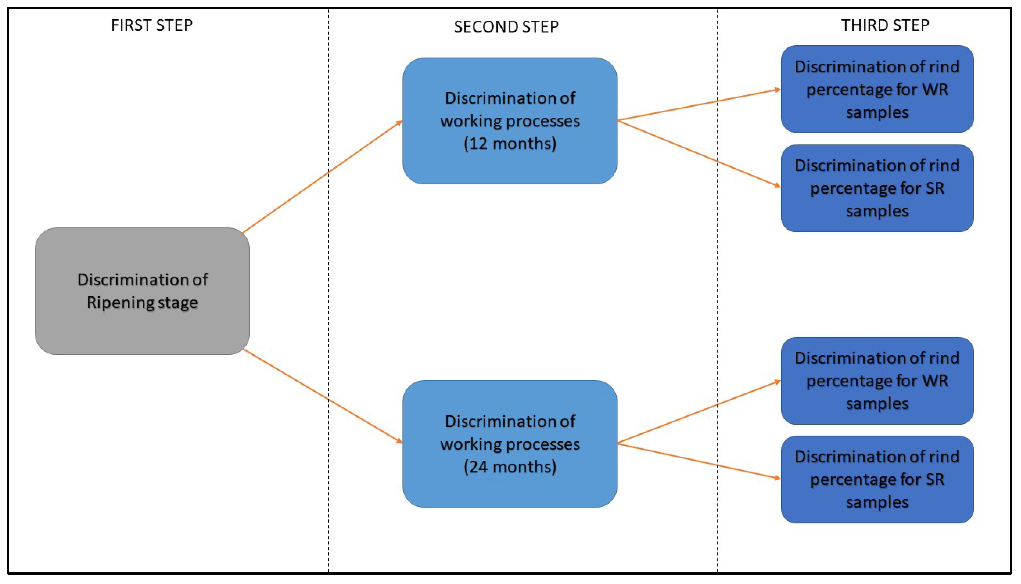
2.1. Samples Preparation and Experimental Design
2.2. GC-MS Analysis
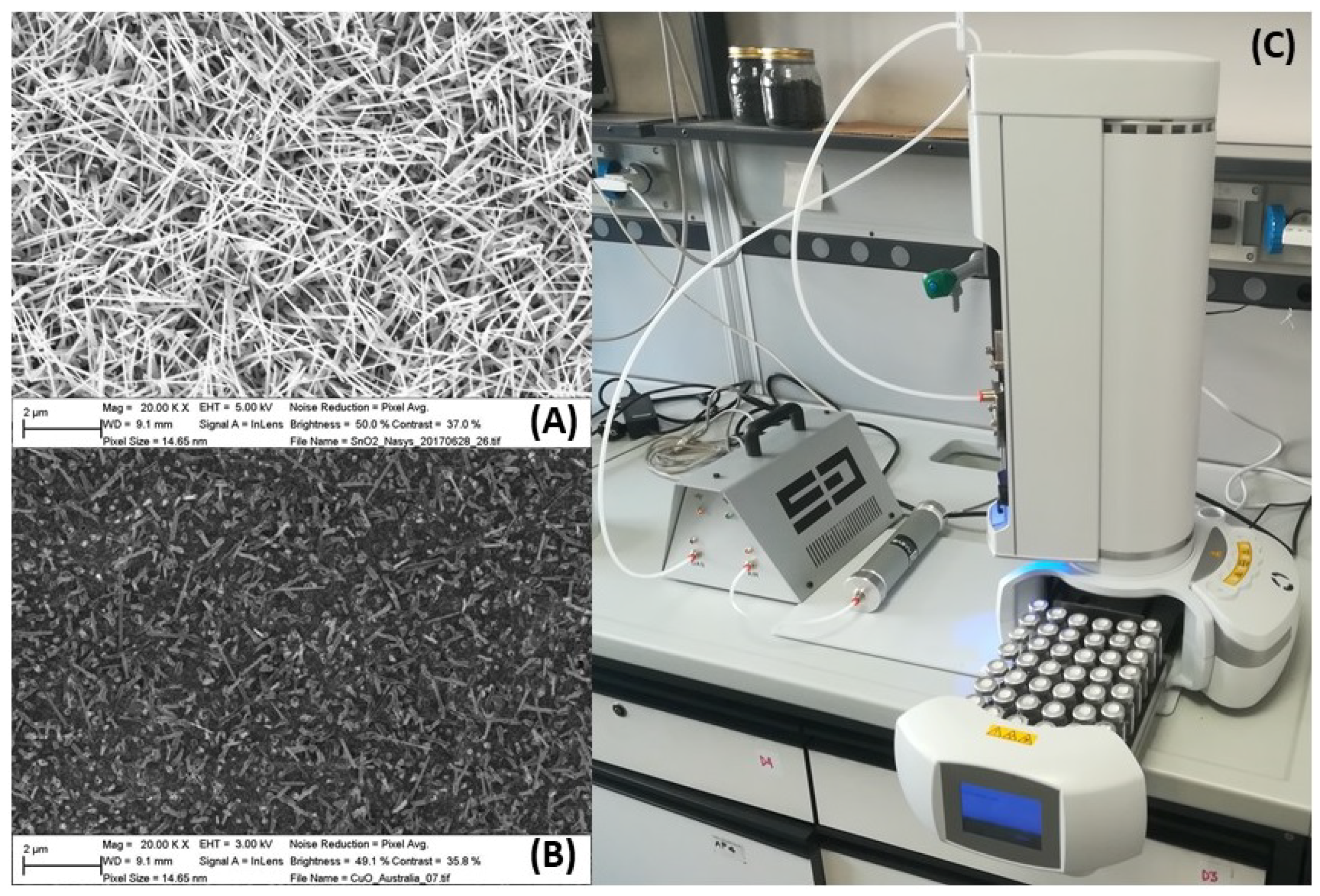
2.3. S3 Analysis
- Injection: the sample HS is flowed in the sensor chamber for 60 s (actual analysis time); then, for 30 s, environmental air flows through the same tube to clean it from any residual VOCs;
- Restore: when the injection period is finished, the filtered air is flowed into the sensors camber. During this time (330 s), the sensors restore the original condition of the base line.
2.4. Data Analysis
3. Results and Discussion
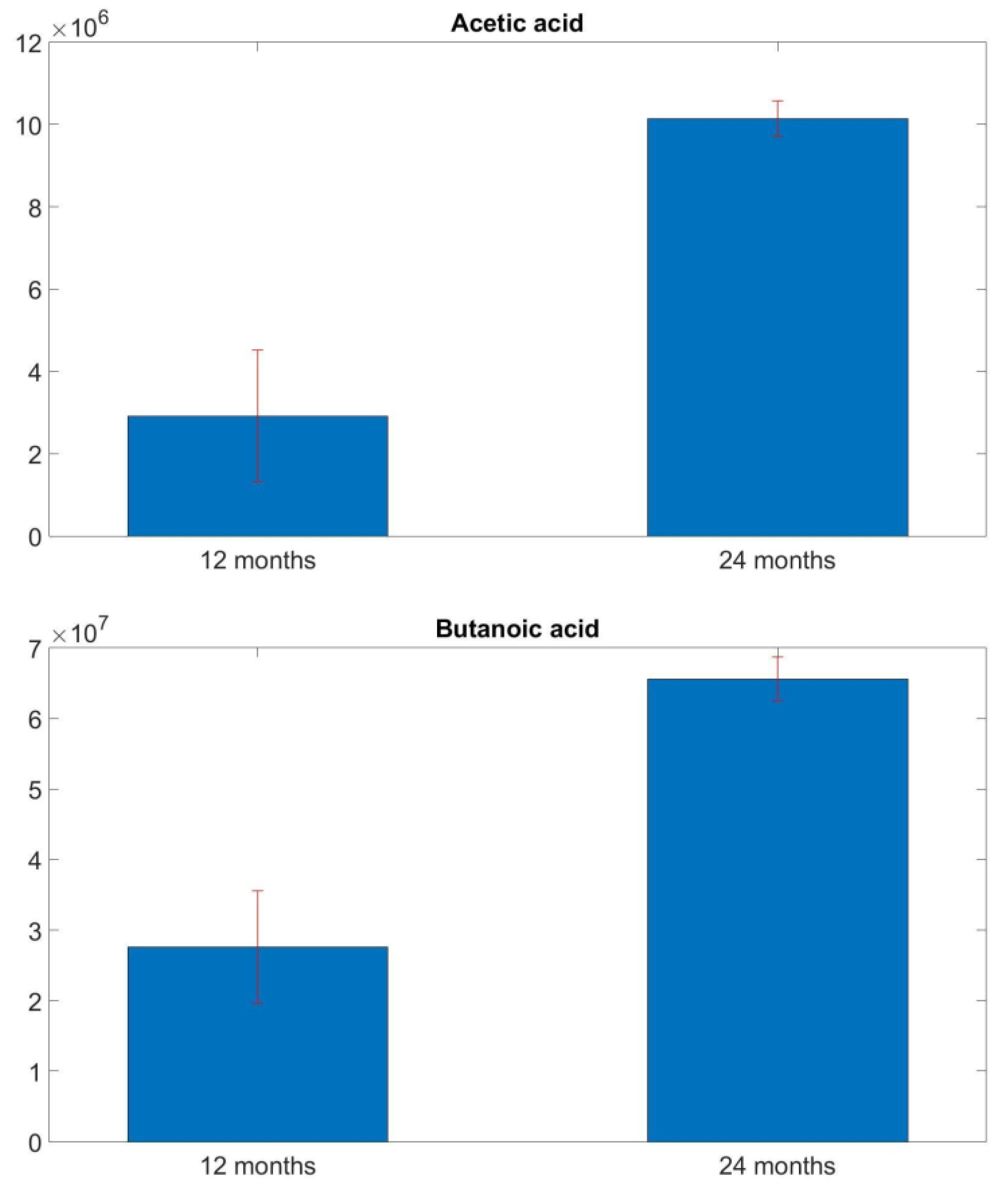
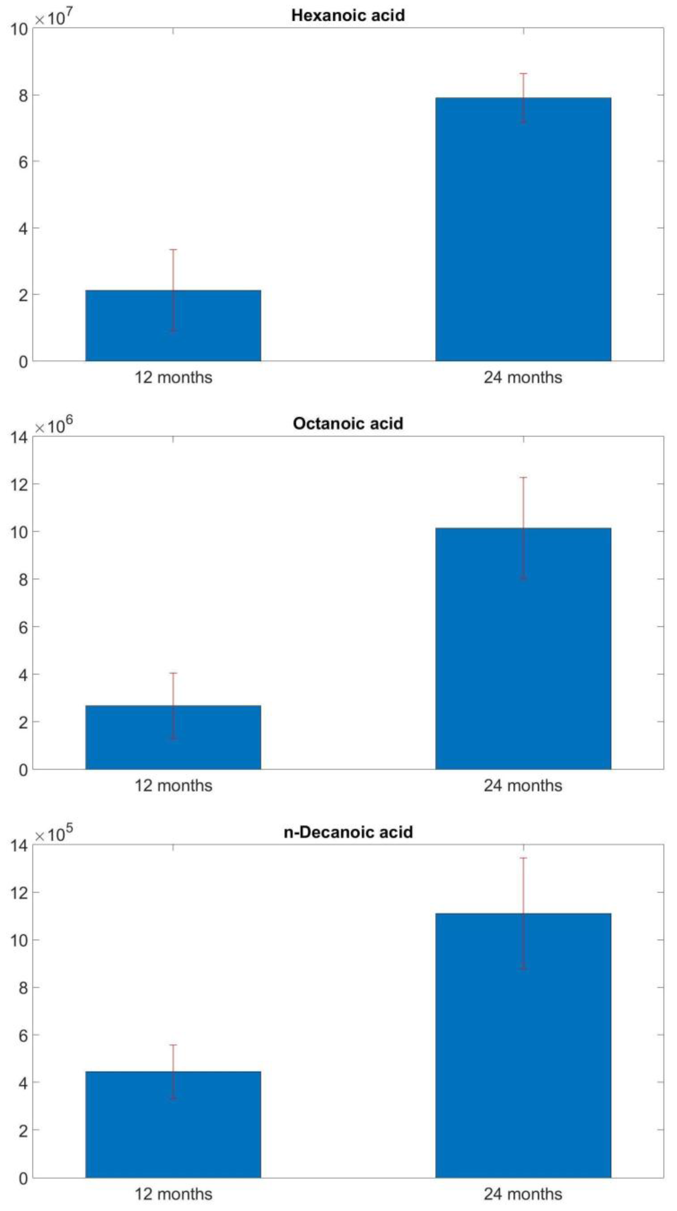
3.1. GC-MS Analysis Results
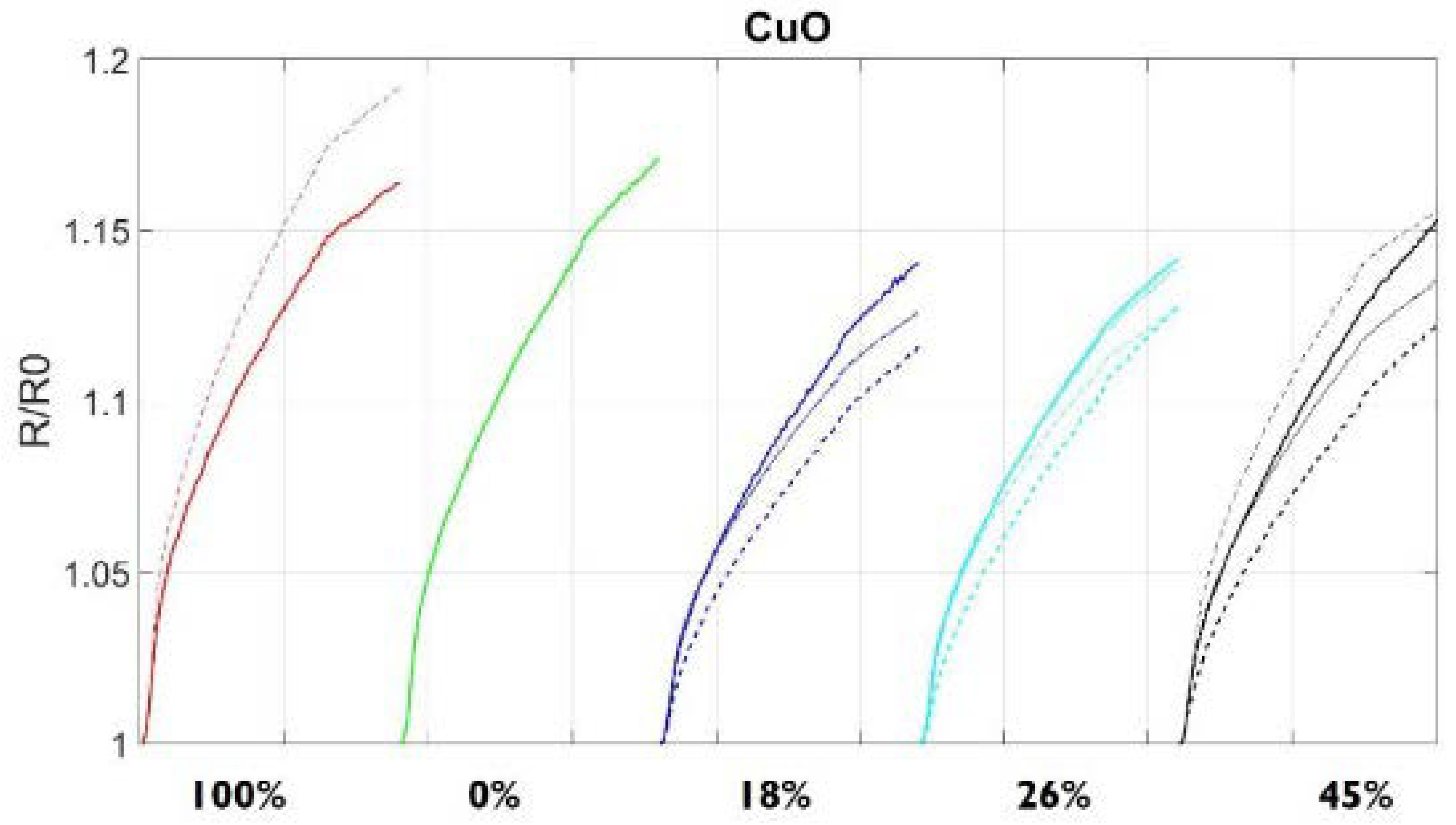
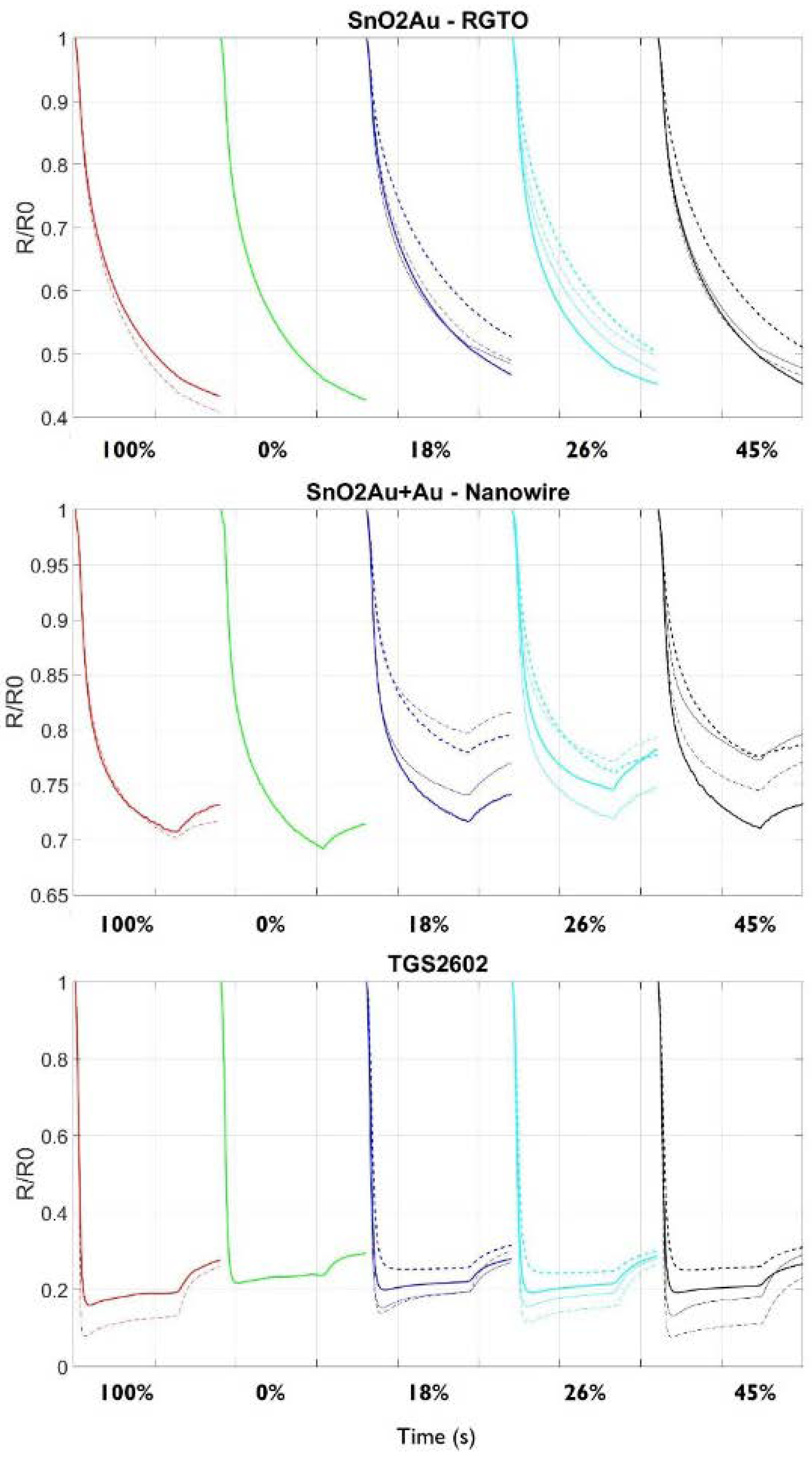
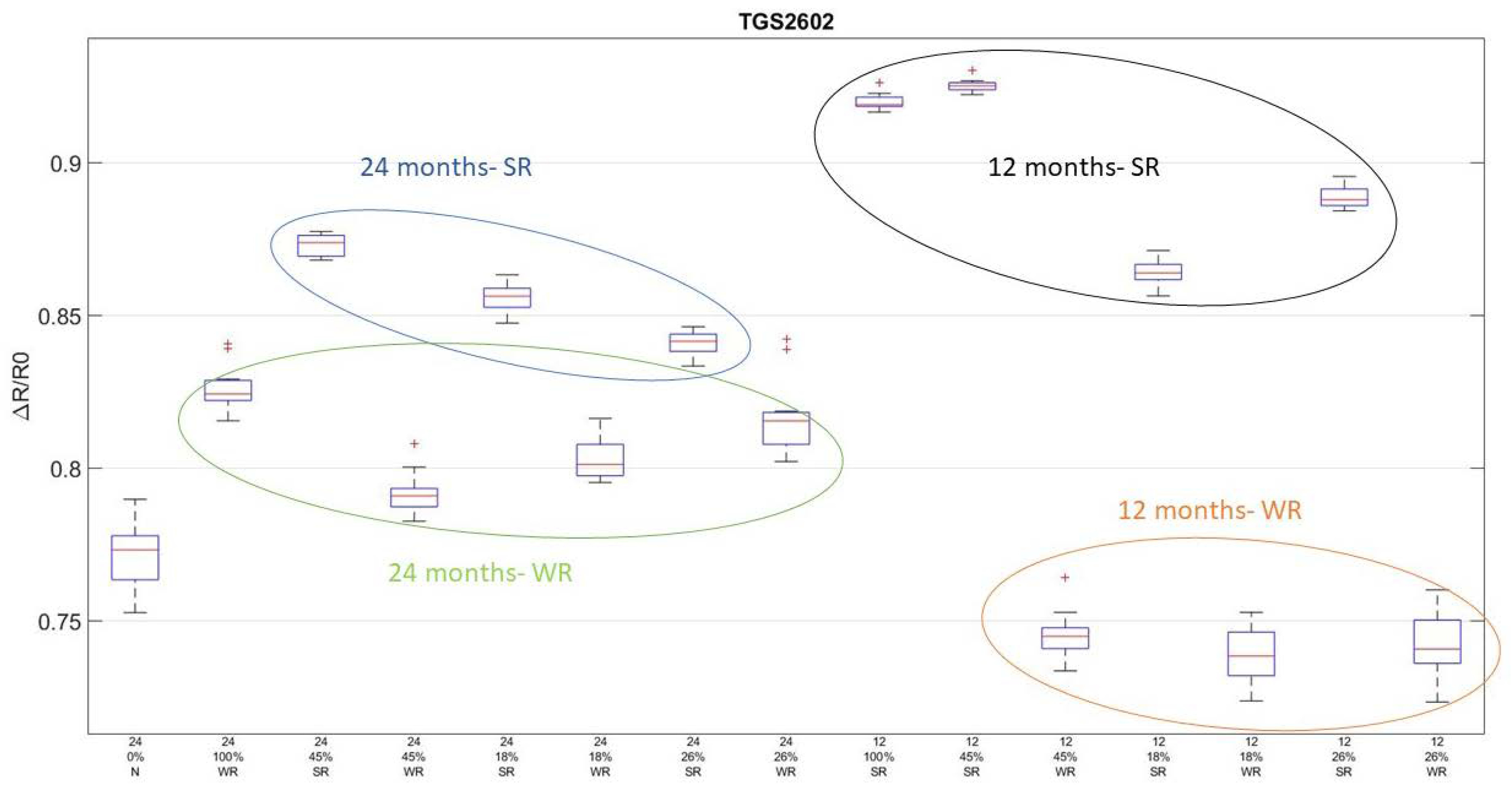
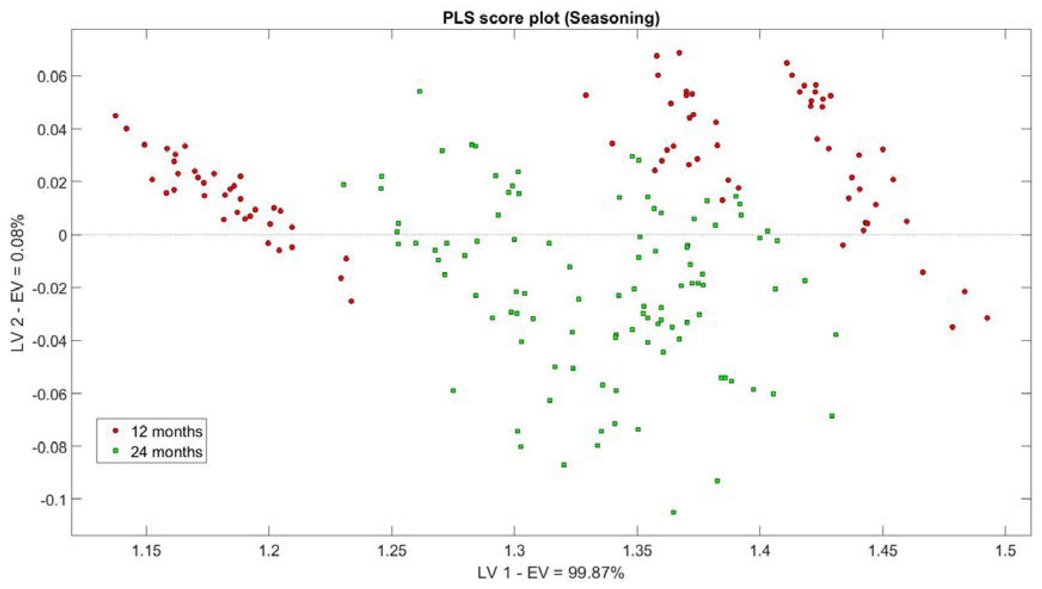
3.2. S3 Analysis Results
4. Conclusions
Author Contributions
Acknowledgments
Conflicts of Interest
References
- Zannoni, M. Evolution of the sensory characteristics of Parmigiano-Reggiano cheese to the present day. Food Qual. Preference 2010, 21, 901–905. [Google Scholar] [CrossRef]
- Caligiani, A.; Nocetti, M.; Lolli, V.; Marseglia, A.; Palla, G. Development of a Quantitative GC-MS Method for the Detection of Cyclopropane Fatty Acids in Cheese as New Molecular Markers for Parmigiano Reggiano Authentication. J. Agric. Food Chem. 2016, 64, 4158–4164. [Google Scholar] [CrossRef] [PubMed]
- Gazzetta Uffiiale. Available online: www.gazzettaufficiale.it/atto/serie_generale/caricaArticolo?art.progressivo=0&art.idArticolo=1&art.versione=1&art.codiceRedazionale=16A06126&art.dataPubblicazioneGazzetta=2016-08-22&art.idGruppo=1&art.idSottoArticolo1=10&art.idSottoArticolo=1&art.flagTipoArticolo=1 (accessed on 27 March 2018).
- Bottari, B.; Quartieri, A.; Prandi, B.; Raimondi, S.; Leonardi, A.; Rossi, M.; Ulrici, A.; Gatti, M.; Sforza, S.; Nocetti, M.; et al. Characterization of the peptide fraction from digested Parmigiano Reggiano cheese and its effect on growth of lactobacilli and bifidobacteria. Int. J. Food Microbiol. 2017, 255, 32–41. [Google Scholar] [CrossRef] [PubMed]
- Malacarne, M.; Summer, A.; Formaggioni, P.; Franceschi, P.; Sandri, S.; Pecorari, M.; Vecchia, P.; Mariani, P. Dairy maturation of milk used in the manufacture of Parmigiano-Reggiano cheese: Effects on physico-chemical characteristics, rennet-coagulation aptitude and rheological properties. J. Dairy Res. 2008, 75, 218–224. [Google Scholar] [CrossRef] [PubMed]
- Sberveglieri, V.; Bhandari, M.P.; Carmona, E.N.; Betto, G.; Sberveglieri, G. A novel MOS nanowire gas sensor device (S3) and GC-MS-based approach for the characterization of grated parmigiano reggiano cheese. Biosensors 2016, 6, 60. [Google Scholar] [CrossRef] [PubMed]
- Popping, B.; De Dominicis, E.; Dante, M.; Nocetti, M. Identification of the Geographic Origin of Parmigiano Reggiano (P.D.O.) Cheeses Deploying Non-Targeted Mass Spectrometry and Chemometrics. Foods 2017, 6, 13. [Google Scholar] [CrossRef] [PubMed]
- Tipologia Grattugiato. Available online: https://www.parmigiano-reggiano.it/consorzio/disciplinare_produzione/tipologia_grattugiato.aspx (accessed on 17 May 2018).
- Maarse, H.; Visscher, C.A. Volatile Compounds in Foods: Qualitative and Quantitative Data; TNO-CIVO Food Analysis Institute: Zeist, The Netherlands, 1989. [Google Scholar]
- Curioni, P.M.G.; Bosset, J.O. Key odorants in various cheese types as determined by gas chromatography-olfactometry. Int. Dairy J. 2002, 12, 959–984. [Google Scholar] [CrossRef]
- Moio, L.; Addeo, F. Grana Padano cheese aroma. J. Dairy Res. 2000, 65, 317–333. [Google Scholar] [CrossRef]
- Qian, M.; Reineccius, G. Identification of Aroma Compounds in Parmigiano-Reggiano Cheese by Gas Chromatography/Olfactometry. J. Dairy Sci. 2002, 85, 1362–1369. [Google Scholar] [CrossRef]
- Carmona, E.N.; Sberveglieri, V.; Comini, E.; Zappa, D.; Pulvirenti, A. Nanowire technology for the detection of microorganisms in potable water. Procedia Eng. 2014, 87, 1453–1456. [Google Scholar] [CrossRef]
- Wilson, A. D Review of Electronic-nose Technologies and Algorithms to Detect Hazardous Chemicals in the Environment. Procedia Technol. 2012, 1, 453–463. [Google Scholar] [CrossRef]
- Wilson, A.D.; Baietto, M. Applications and Advances in Electronic-Nose Technologies. Sensors 2009, 9, 5099–5148. [Google Scholar] [CrossRef] [PubMed]
- Muñoz, R.; Sivret, E.C.; Parcsi, G.; Lebrero, R.; Wang, X.; Suffet, I.H.; Stuetz, R.M. Monitoring techniques for odour abatement assessment. Water Res. 2010, 44, 5129–5149. [Google Scholar] [CrossRef] [PubMed]
- Gębicki, J.; Dymerskib, T.; Namieśnik, J. Monitoring of Odour Nuisance from Landfill Using Electronic Nose. Chem. Eng. Trans. 2014, 40, 85–90. [Google Scholar] [CrossRef]
- D’Amico, A.; Pennazza, G.; Santonico, M.; Martinelli, E.; Roscioni, C.; Galluccio, G.; Paolesse, R.; Di Natale, C. An investigation on electronic nose diagnosis of lung cancer. Lung Cancer 2010, 68, 170–176. [Google Scholar] [CrossRef] [PubMed]
- Dutta, R.; Morgan, D.; Baker, N.; Gardner, J.W.; Hines, E.L. Identification of Staphylococcus aureus infections in hospital environment: Electronic nose based approach. Sens. Actuators B Chem. 2005, 109, 355–362. [Google Scholar] [CrossRef]
- Pavlou, A.K.; Magan, N.; McNulty, C.; Jones, J.M.; Sharp, D.; Brown, J.; Turner, A.P.F. Use of an electronic nose system for diagnoses of urinary tract infections. Biosens. Bioelectron. 2002, 17, 893–899. [Google Scholar] [CrossRef]
- Kodogiannis, V.S.; Lygouras, J.N.; Tarczynski, A.; Chowdrey, H.S. Artificial Odor Discrimination System Using Electronic Nose and Neural Networks for the Identification of Urinary Tract Infection. IEEE Trans. Inf. Technol. Biomed. 2008, 12, 707–713. [Google Scholar] [CrossRef] [PubMed]
- Covington, J.A.; Westenbrink, E.W.; Ouaret, N.; Harbord, R.; Bailey, C.; O’Connel, N.; Cullis, J.; Williams, N.; Nwokolo, C.; Bardhan, K.D.; et al. Application of a Novel Tool for Diagnosing BIle Acid Diarrhoea. Sensors 2013, 13, 11899–11912. [Google Scholar] [CrossRef] [PubMed]
- Loutfi, A.; Coradeschi, S.; Mani, G.K.; Shankar, P.; Rayappan, J.B.B. Electronic Noses for Food Quality: A Review. J. Food Eng. 2014, 144, 103–111. [Google Scholar] [CrossRef]
- Macias, M.M.; Agudo, J.E.; Manso, A.G.; Orellana, C.J.G.; Velasco, H.M.G.; Caballero, R.G. A Compact and Low Cost Electronic Nose for Aroma Detection. Sensors 2013, 13, 5528–5541. [Google Scholar] [CrossRef] [PubMed]
- Wojnowski, W.; Majchrzak, T.; Dymerski, T.; Gębicki, J.; Namieśnik, J. Portable Electronic Nose Based on Electrochemical Sensors for Food Quality Assessment. Sensors 2017, 17, 2715. [Google Scholar] [CrossRef] [PubMed]
- Sberveglieri, V.; Falasconi, M.; Gobbi, E.; Carmona, E.N.; Zambotti, G.; Pulvirenti, A. Candida milleri detected by Electronic noce in tomato sauce. Procedia Eng. 2014, 87, 584–587. [Google Scholar] [CrossRef]
- Sberveglieri, V.; Comini, E.; Zappa, D.; Pulvirenti, A.; Carmona, E.N. Electronic nose for the early detection of different types of indigenous mold contamination in green coffee. In Proceedings of the 2013 Seventh International Conference on Sensing Technology (ICST), Wellington, New Zealand, 3–5 December 2013; pp. 461–465. [Google Scholar] [CrossRef]
- Labreche, S.; Bazzo, S.; Cade, S.; Chanie, E. Shelf life determination by electronic nose: Application to milk. Sens. Actuators B 2005, 106, 19–206. [Google Scholar] [CrossRef]
- Qiu, S.; Wang, J. The prediction of food additives in the fruit juice based on electronic nose with chemometrics. Food Chem. 2017, 230, 208–214. [Google Scholar] [CrossRef] [PubMed]
- Baietto, M.; Wilson, A.D. Electronic-Nose Applications for Fruit Identification, Ripeness and Quality Grading. Sensors 2015, 15, 899–931. [Google Scholar] [CrossRef] [PubMed]
- Gursoy, O.; Somervuo, P.; Alatossava, T. Preliminary study of ion mobility based electronic nose GD-1 for discrimination of hard cheeses. J. Food Eng. 2009, 92, 202–207. [Google Scholar] [CrossRef]
- Pais, V.F.; Oliveira, J.A.B.P.; Gomes, M.T.S.R. An Electronic Nose Based on Coated Piezoelectric Quartz Crystals to Certify Ewes’ Cheese and to Discriminate between Cheese Varieties. Sensors 2012, 12, 1422–1436. [Google Scholar] [CrossRef] [PubMed]
- Marsili, R.T. Comparison of solid-phase microextraction and dynamic headspace methods for the gas chromatographic-mass spectrometric analysis of light-induced lipid oxidation products in milk. J. Chromatogr. Sci. 1999, 37, 17–23. [Google Scholar] [CrossRef] [PubMed]
- Shooter, D.; Jayatissa, N.; Renner, N. Volatile reduced sulphur compounds in butter by solid phase microextraction. J. Dairy Res. 1999, 66, 115–123. [Google Scholar] [CrossRef]
- Frank, D.C.; Owen, C.M.; Patterson, J. Solid phase microextraction (SPME) combined with gas-chromatography and olfactometry-mass spectrometry for characterization of cheese aroma compounds. LWT Food Sci. Technol. 2004, 37, 139–154. [Google Scholar] [CrossRef]
- Peres, C.; Viallon, C.; Berdague, J. Solid-Phase Microextraction-Mass Spectrometry: A New Approach to the Rapid Characterization of Cheeses. Anal. Chem. 2001, 73, 1030–1036. [Google Scholar] [CrossRef] [PubMed]
- Ponzoni, A.; Zappa, D.; Comini, E.; Sberveglieri, V.; Faglia, G.; Sberveglieri, G. Metal oxide nanowire gas sensors: Application of conductometric and surface ionization architectures. Chem. Eng. Trans. 2012, 30, 31–36. [Google Scholar] [CrossRef]
- Sberveglieri, G.; Concina, I.; Comini, E.; Falasconi, M.; Ferroni, M.; Sberveglieri, V. Synthesis and integration of tin oxide nanowires into an electronic nose. Vacuum 2012, 86, 532–535. [Google Scholar] [CrossRef]
- Wagner, R.S.; Ellis, W.C. Vapor-Liquid-Solid Mechanism of Single Crystal Growth. Appl. Phys. Lett. 1964, 4, 89–90. [Google Scholar] [CrossRef]
- Carmona, E.N.; Sberveglieri, V.; Ponzoni, A.; Zappa, D.; Pulvirenti, A. Detection of microbial contamination in potable water by Nanowire technology. In Proceedings of the 8th International Conference on Sensing Technology, Liverpool, UK, 2–4 September 2014. [Google Scholar]
- Botelho, B.G.; Reis, N.; Oliveira, L.S.; Sena, M.M. Development and analytical validation of a screening method for simultaneous detection of five adulterants in raw milk using mid-infrared spectroscopy and PLS-DA. Food Chem. 2015, 181, 31–37. [Google Scholar] [CrossRef] [PubMed]
- Lenhardt, L.; Bro, R.; Zeković, I.; Dramićanin, T.; Dramićanin, M.D. Fluorescence spectroscopy coupled with PARAFAC and PLS DA for characterization and classification of honey. Food Chem. 2015, 175, 284–291. [Google Scholar] [CrossRef] [PubMed]
- Cozzolino, D.; Smyth, H.E.; Cynkar, W.; Dambergs, R.G.; Gishen, M. Usefulness of chemometrics and mass spectrometry-based electronic nose to classify Australian white wines by their varietal origin. Talanta 2005, 68, 382–387. [Google Scholar] [CrossRef] [PubMed]
- Consonni, R.; Cagliani, L.R. Ripening and geographical characterization of Parmigiano Reggiano cheese by 1H NMR spectroscopy. Talanta 2008, 76, 200–205. [Google Scholar] [CrossRef] [PubMed]
- Wang, S.C. Artificial Neural Network. In Interdisciplinary Computing in Java Programming; The Springer International Series in Engineering and Computer Science; Springer: Boston, MA, USA, 2003; Volume 743. [Google Scholar]
- Yu, H.; Wang, J.; Yao, C.; Zhang, H.; Yu, Y. Quality grade identification of green tea using E-nose by CA and ANN. LWT Food Sci. Technol. 2008, 41, 1268–1273. [Google Scholar] [CrossRef]
- Berrueta, L.A.; Alonso-Salces, R.M.; Heberger, K. Supervised pattern recognition in food analysis. J. Chromatogr. A 2007, 1158, 196–214. [Google Scholar] [CrossRef] [PubMed]
- Tan, J.; Kerr, W. L Determining Degree of Roasting in Cocoa Beans by Artificial Neural Network (ANN) based Electronic Nose System and Gas Chromatography/Mass Spectrometry (GC/MS). J. Sci. Food Agric. 2018. [Google Scholar] [CrossRef] [PubMed]
- Adak, M.F.; Yumusak, N. Classification of E-Nose Aroma Data of Four Fruit Types by ABC-Based Neural Network. Sensors 2016, 16, 304. [Google Scholar] [CrossRef] [PubMed]
- Ballabio, D.; Consonni, V. Classification tools in chemistry. Part 1: Linear models. PLS-DA. Anal. Methods 2013, 5, 3790–3798. [Google Scholar] [CrossRef]
- Tosi, F.; Sandri, S.; Tedeschi, G.; Malacarne, M.; Fossa, E. Variazioni di composizione e prprietà fisico-chimiche del Parmigiano Reggiano durante la maturazione e in differenti zone della forma. Sci. Tec. Latt. Casearia 2008, 59, 507–528. [Google Scholar]
- Nanni, M.; Coppola, R.; Iorizzo, M.; Sorrentino, A.; Sorrentino, E.; Grazia, L. La microflora lattica nella maturazione del formaggio Parmigiano Reggiano. Sci. Tec. Latt. Casearia 1997, 48, 211–216. [Google Scholar]
- 2-Nonanone. Available online: https://pubchem.ncbi.nlm.nih.gov/compound/2-nonanone (accessed on 29 March 2018).
- Jollivet, N.; Chataud, J.; Vayssier, Y.; Bensoussan, M. Production of volatile compounds in model milk and cheese media by eight strains of Geotrichum candidum. J. Dairy Res. 1994, 61, 241–248. [Google Scholar] [CrossRef]
- Jou, K.D.; Harper, W.J. Pattern recognition of Swiss cheese aroma compounds by SPME/GC and an electronic nose. Milchwissenschaft 1998, 53, 259–263. [Google Scholar]
- Pillonel, L.; Ampuero, S.; Tabacchi, R.; Bosset, J.O. Analytical methods for the determination of the geographic origin of Emmental cheese, Volatile compounds by GC-MS-FID and electronic nose. Eur. J. Food Res. Technol. 2003, 216, 179–183. [Google Scholar] [CrossRef]
- Schaller, E.; Bosset, J.O.; Escher, F. Feasibility study: Detection of rind taste off-flavour in Swiss Emmental cheese using an electroinc nose and a GC-MS. Mitt. Lebensm. Hyg. 2000, 91, 610–615. [Google Scholar]
- Sberveglieri, V. Validation of Parmigiano Reggiano Cheese Aroma Authenticity, Categorized through the Use of an Array of Semiconductors Nanowire Device (S3). Materials 2016, 9, 81. [Google Scholar] [CrossRef] [PubMed]


| Materials (Type) | Composition | Morphology | Operating Temperature (°C) | Response to 5 ppm of Ethanol | Selectivity | Limit of Detection (LOD) of Ethanol (ppm) |
|---|---|---|---|---|---|---|
| SnO2Au (n) | SnO2 functionalized with Au clusters | RGTO | 400 °C | 6.5 | 3 | 0.5 |
| SnO2 (n) | SnO2 | RGTO | 300 °C | 3.5 | 2.5 | 1 |
| SnO2 (n) | SnO2 | RGTO | 400 °C | 4 | 2 | 0.8 |
| SnO2Au+Au (n) | SnO2 grown with Au and functionalized with gold clusters | Nanowire | 350 °C | 7 | 2.5 | 0.5 |
| SnO2Au (n) | SnO2 grown with Au | Nanowire | 350 °C | 5 | 2.1 | 1 |
| CuO (p) | CuO | Nanowire | 400 °C | 1.5 | 1.5 | 1 |
| SeasoningPercentage | 0% | 18% | 26% | 45% | 100% | ||||
|---|---|---|---|---|---|---|---|---|---|
| WR | SR | WR | SR | WR | SR | WR | SR | ||
| 12 months | - | 11 | 12 | 13 | 11 | 12 | 14 | - | 14 |
| 24 months | 12 | 14 | 14 | 13 | 13 | 11 | 13 | 13 | - |
| First Step Ripening Stage | Second Step Working Processes | Third Step Rind Percentage | |
|---|---|---|---|
| PLD-DA | 94.7% | 12 months: 100% | WR: 61.1% |
| SR: 90.2% | |||
| 24 months: 79% | WR:90.2% | ||
| SR: 95% | |||
| ANN | 100% | 12 months: 100% | WR: 63.8% |
| SR: 96.1% | |||
| 24 months: 100% | WR: 58.8% | ||
| SR: 100% |
© 2018 by the authors. Licensee MDPI, Basel, Switzerland. This article is an open access article distributed under the terms and conditions of the Creative Commons Attribution (CC BY) license (http://creativecommons.org/licenses/by/4.0/).
Share and Cite
Abbatangelo, M.; Núñez-Carmona, E.; Sberveglieri, V.; Zappa, D.; Comini, E.; Sberveglieri, G. Application of a Novel S3 Nanowire Gas Sensor Device in Parallel with GC-MS for the Identification of Rind Percentage of Grated Parmigiano Reggiano. Sensors 2018, 18, 1617. https://doi.org/10.3390/s18051617
Abbatangelo M, Núñez-Carmona E, Sberveglieri V, Zappa D, Comini E, Sberveglieri G. Application of a Novel S3 Nanowire Gas Sensor Device in Parallel with GC-MS for the Identification of Rind Percentage of Grated Parmigiano Reggiano. Sensors. 2018; 18(5):1617. https://doi.org/10.3390/s18051617
Chicago/Turabian StyleAbbatangelo, Marco, Estefanía Núñez-Carmona, Veronica Sberveglieri, Dario Zappa, Elisabetta Comini, and Giorgio Sberveglieri. 2018. "Application of a Novel S3 Nanowire Gas Sensor Device in Parallel with GC-MS for the Identification of Rind Percentage of Grated Parmigiano Reggiano" Sensors 18, no. 5: 1617. https://doi.org/10.3390/s18051617
APA StyleAbbatangelo, M., Núñez-Carmona, E., Sberveglieri, V., Zappa, D., Comini, E., & Sberveglieri, G. (2018). Application of a Novel S3 Nanowire Gas Sensor Device in Parallel with GC-MS for the Identification of Rind Percentage of Grated Parmigiano Reggiano. Sensors, 18(5), 1617. https://doi.org/10.3390/s18051617