An Effective Delay Reduction Approach through a Portion of Nodes with a Larger Duty Cycle for Industrial WSNs


 ,
,  and
and
Abstract
:1. Introduction
- (1)
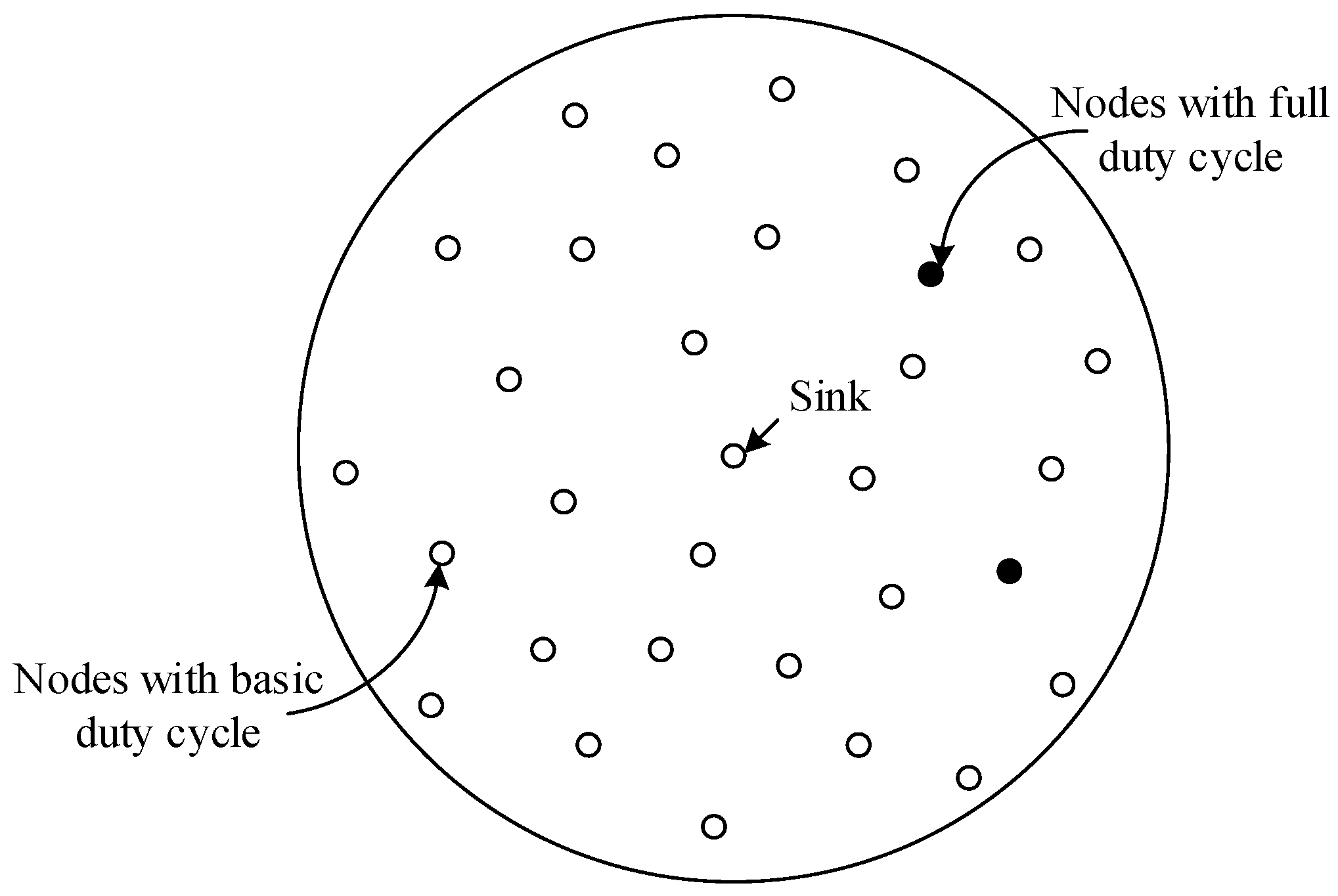
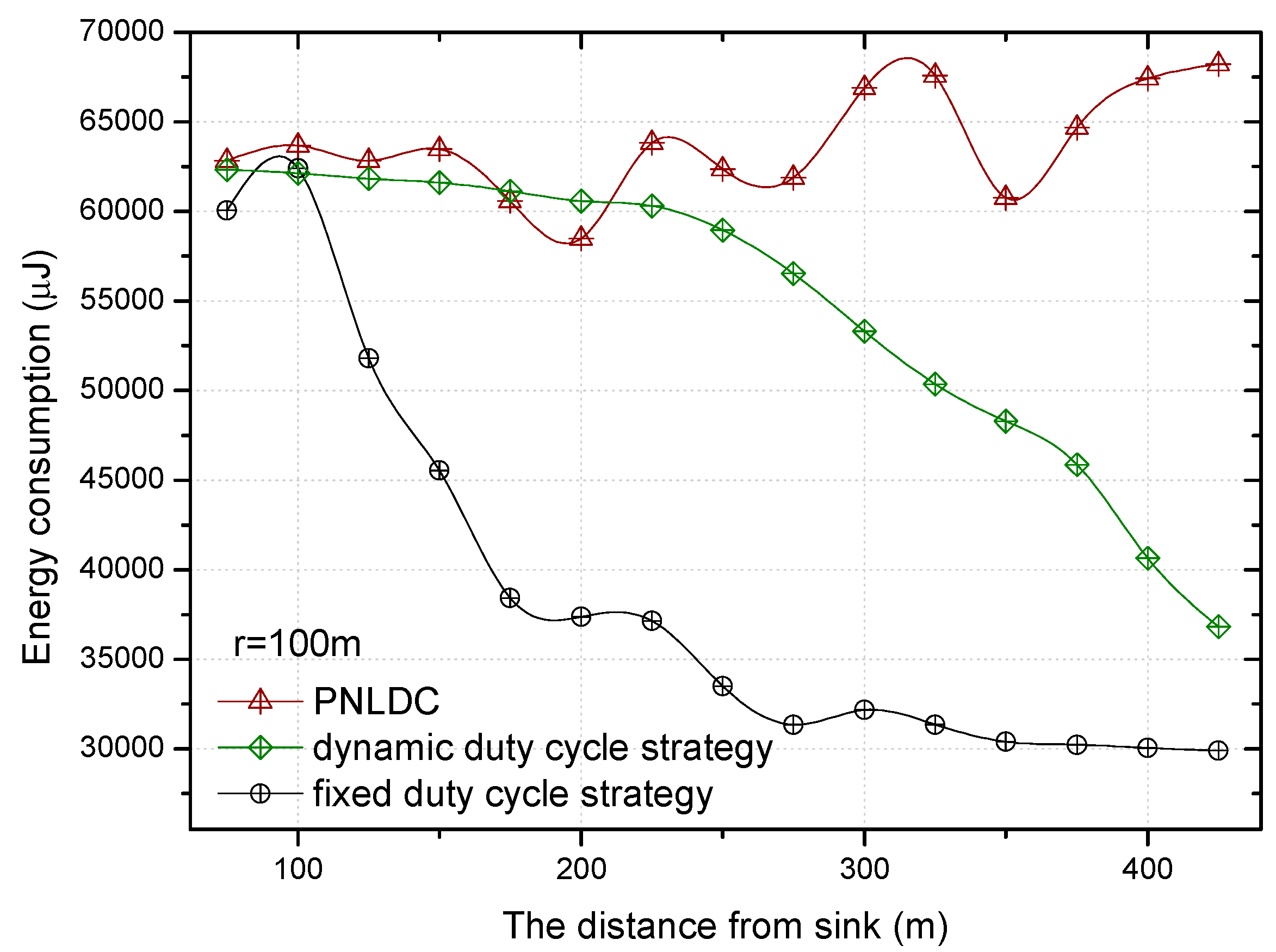
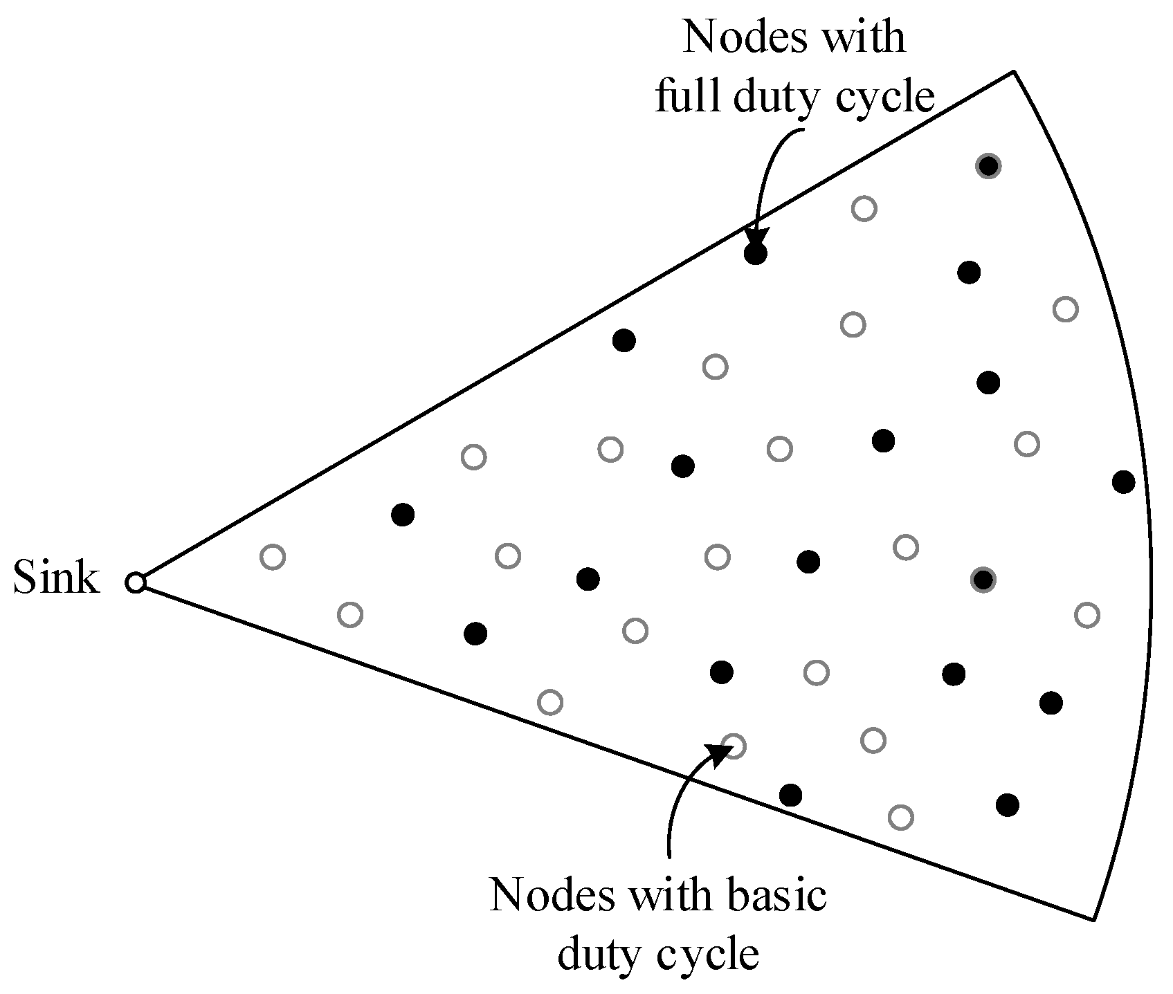
- A novel Portion of Nodes with Larger Duty Cycle (PNLDC) scheme is proposed to reduce sleep delay and maintain a high lifetime for IWSNs. We have taken note of the following two facts: First, the sender has multiple forwarding nodes and the sleep delay is equal to 0 as long as the duty cycle of any node in the forwarding nodes set (FNS) is 1. Second, a significant number of studies show that the nodes in the near sink region bear a lot of data so their energy consumption is high while the nodes far away from the sink have residual energy. Therefore, a PNLDC scheme makes full use of the residual energy of non-hotspots to set the duty cycle of a certain proportion of nodes to 1 (). Thus, a PNLDC scheme is able to reduce delay while ensuring that lifetime is not less than the previous strategy.
- (2)
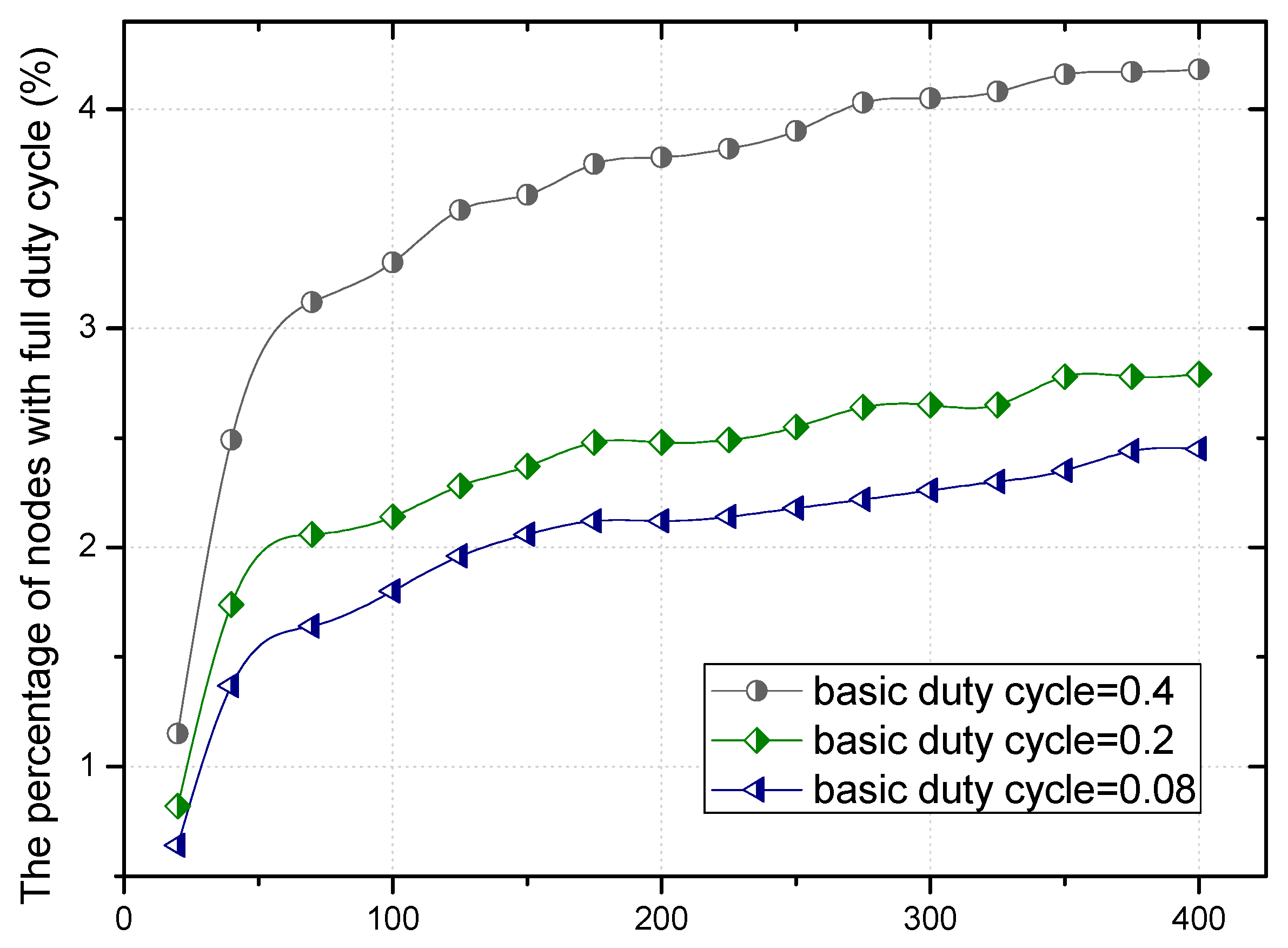
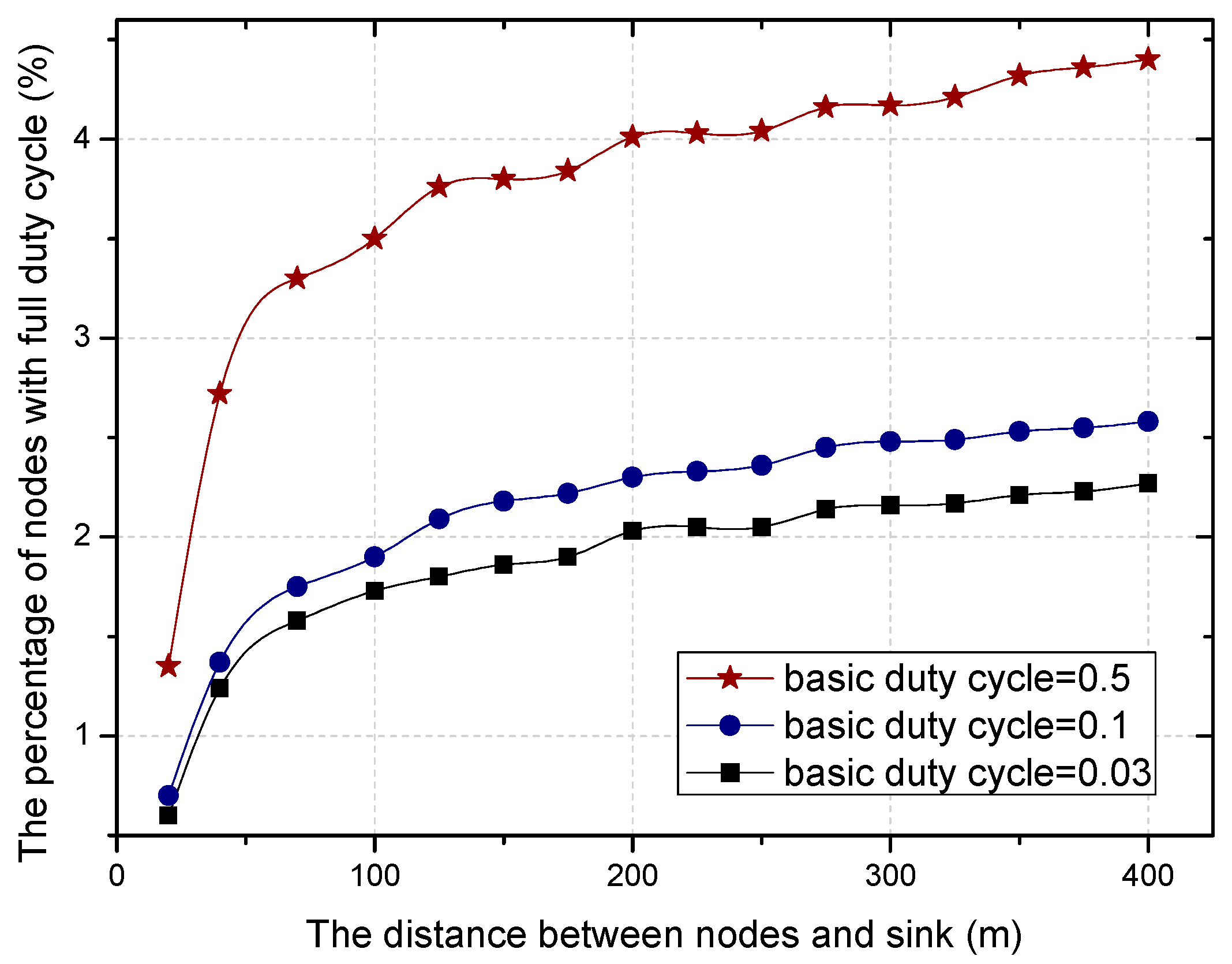
- Through strict theoretical calculation and deduction, this paper first gives the proportion of nodes with full duty cycle (duty cycle = 1) in different regions that have different distances to the sink. Then, the relationship between the proportion of nodes with full duty cycle and the reduced delay is given. This provides the theoretical basis for the PNLDC strategy and provides the basis for the calculation of similar methods.
- (3)
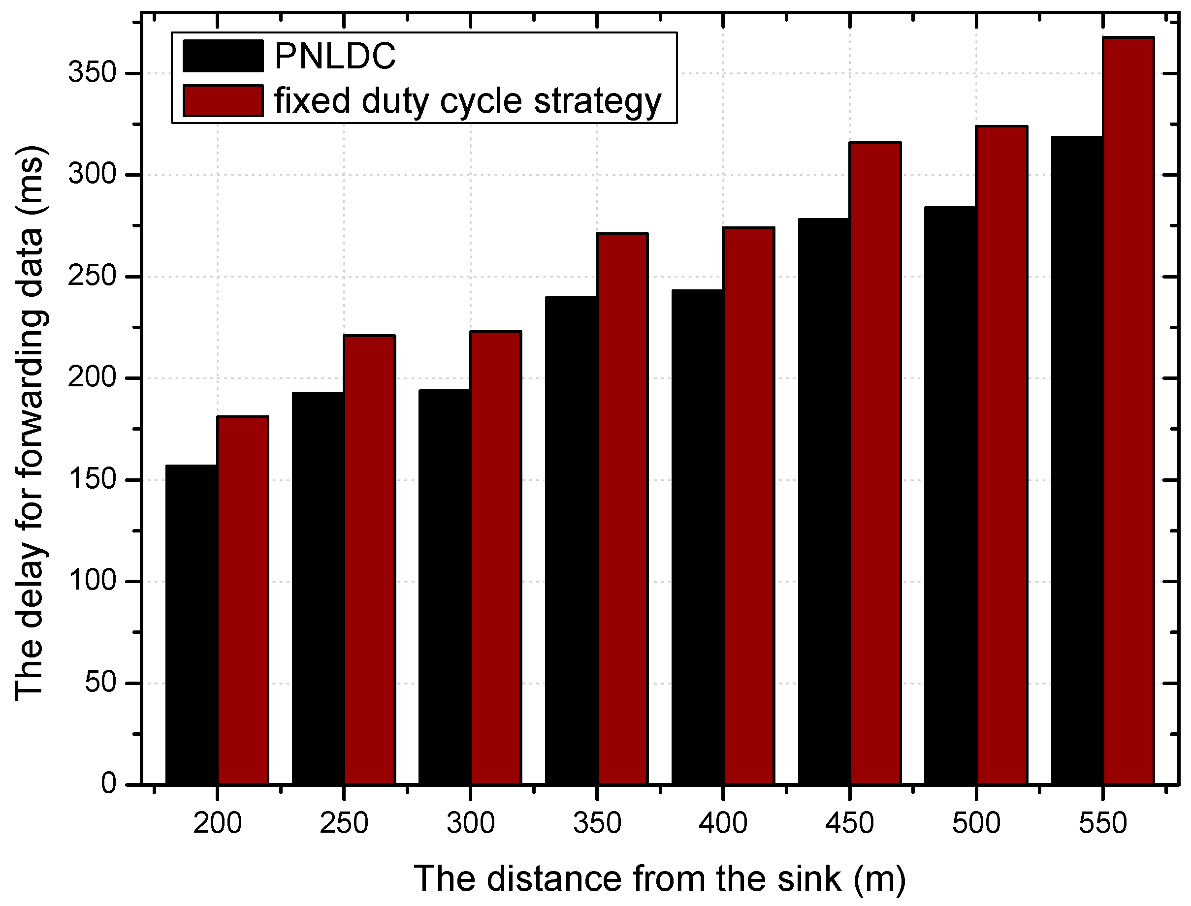
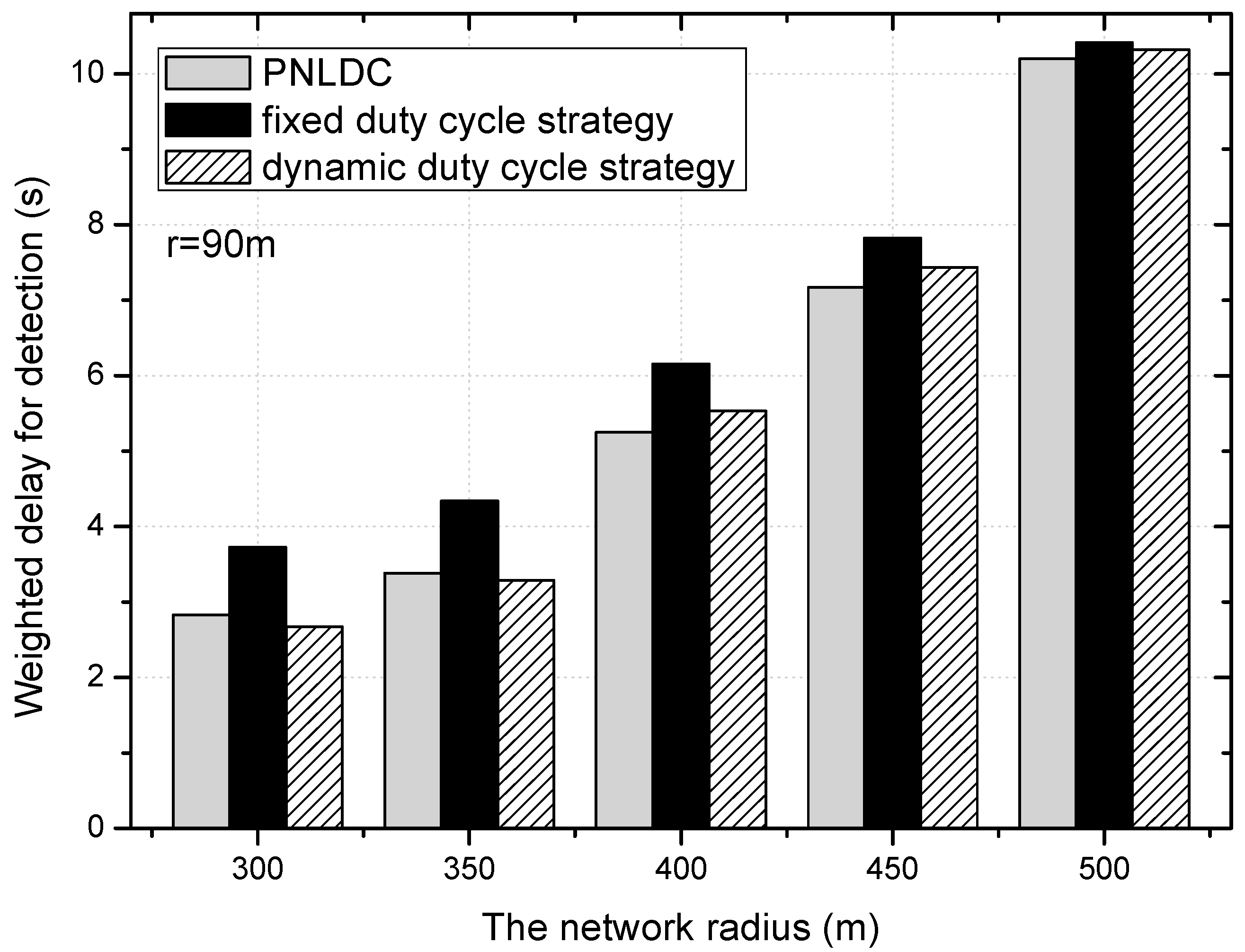
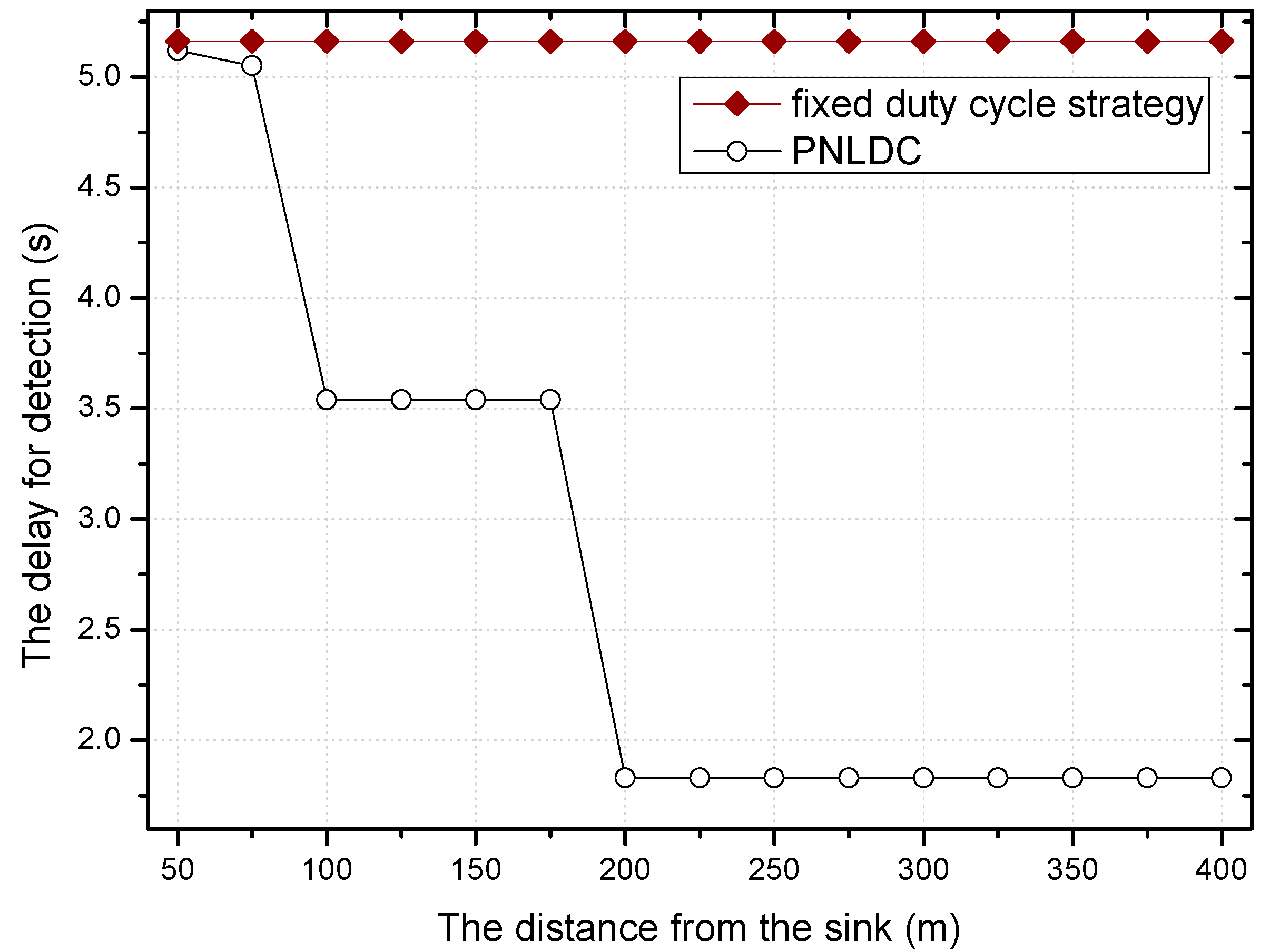
- The full theoretical analysis in this paper shows that the proposed PNLDC scheme significantly reduces the delay for forwarding data by 8.9~26.4% and delay for detection by 2.1~24.6% without reducing the network lifetime when compared to the fixed duty cycle approach.
2. Related Work
3. System Model and Problem Statements
3.1. System Model
3.2. System Parameters
3.3. Problem Statements
4. The Design of PNLDC Approach
4.1. Research Motivation
4.2. The PNLDC Approach Design
5. Performance Analysis and Simulation Results
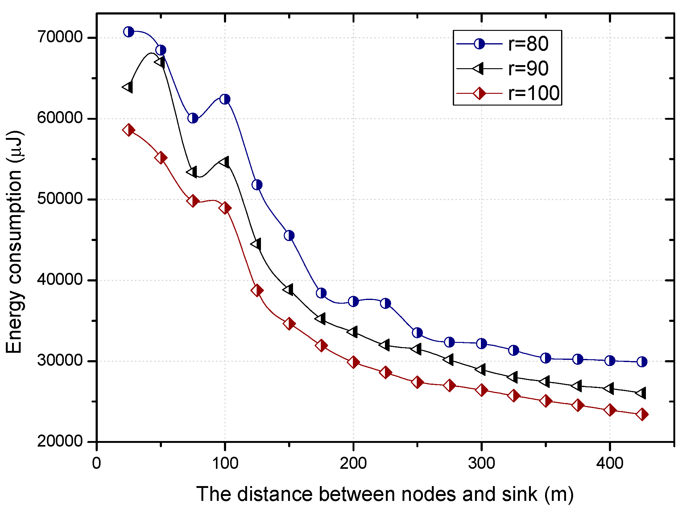
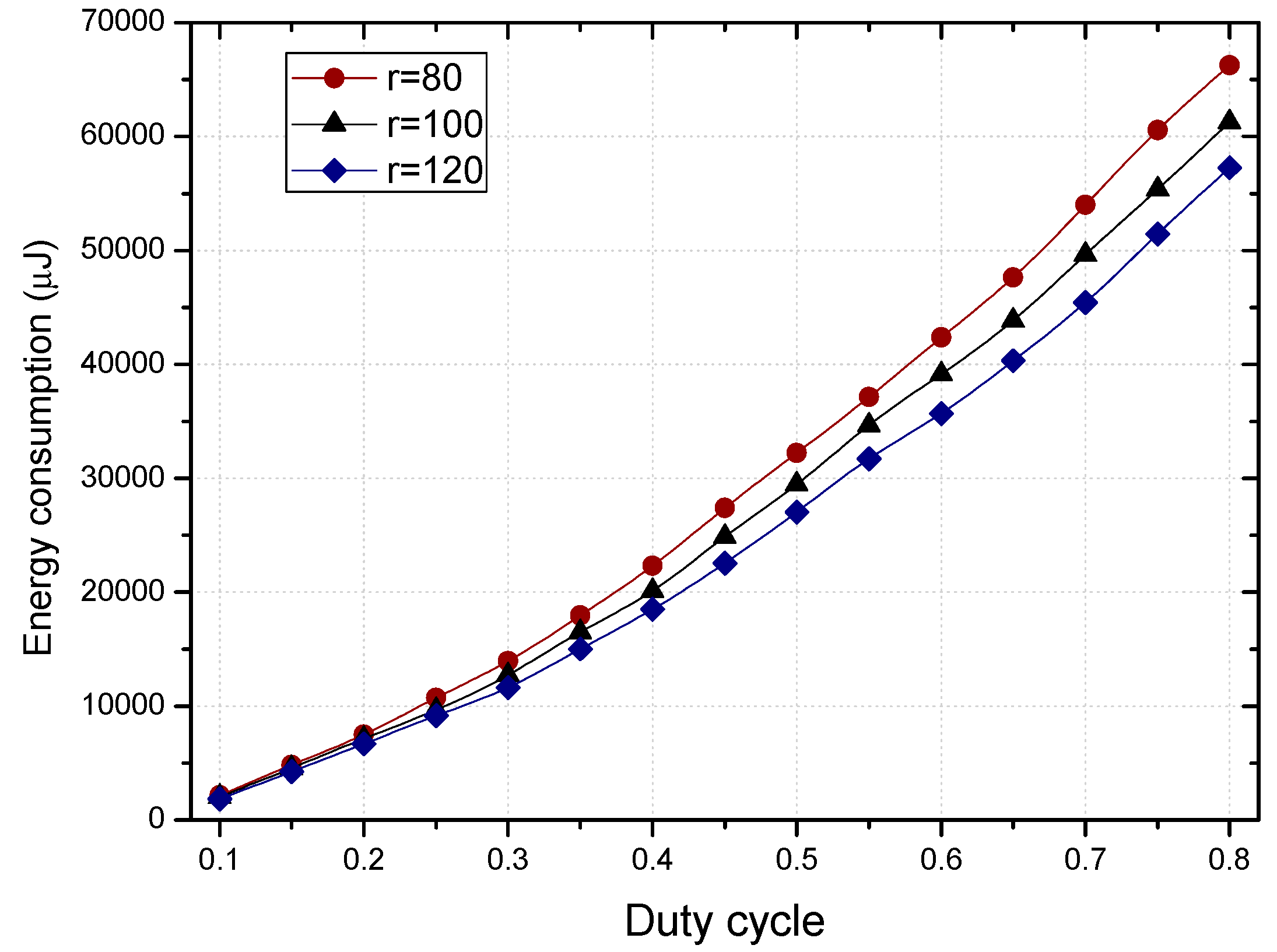
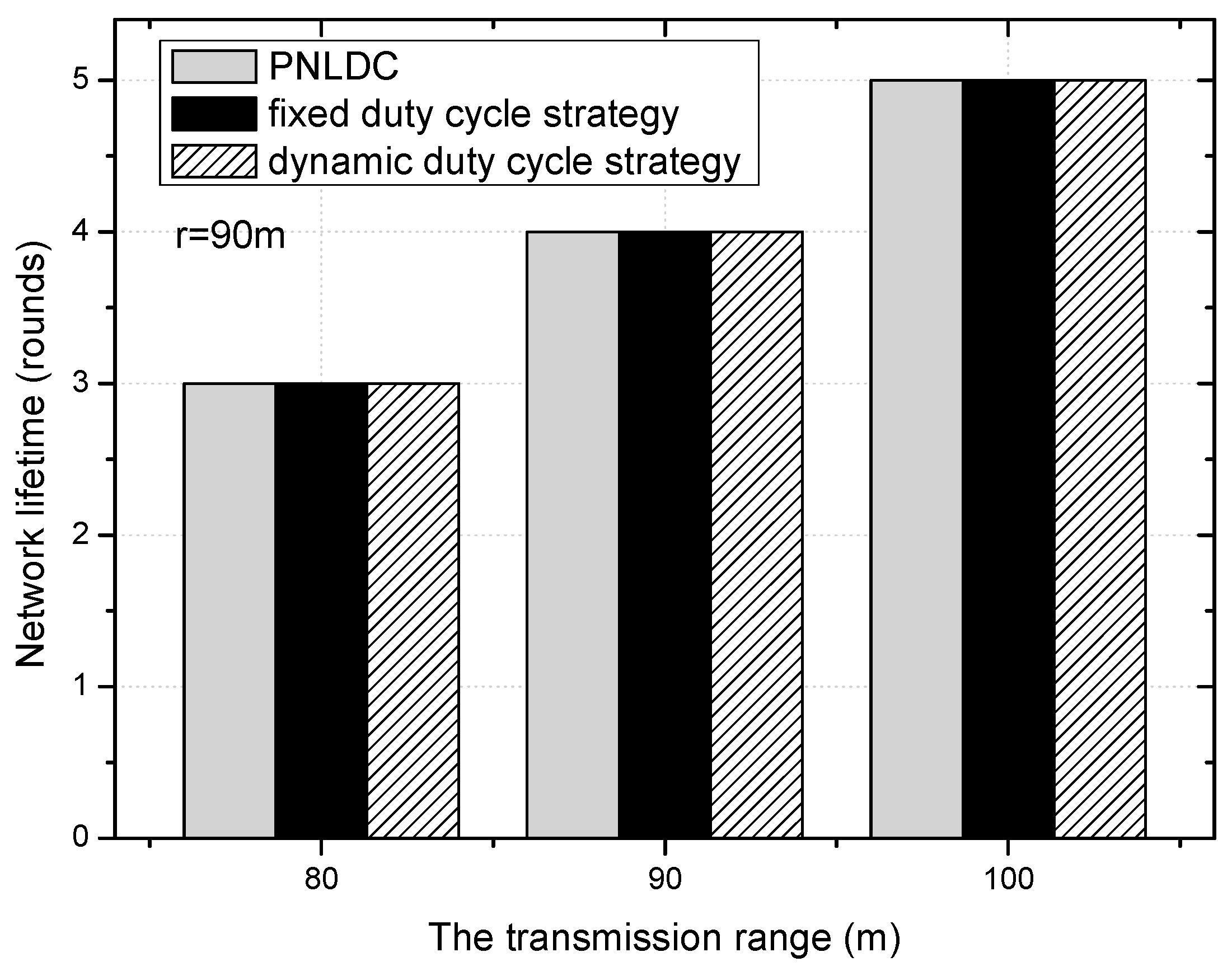
5.1. Energy Consumption and Network Lifetime
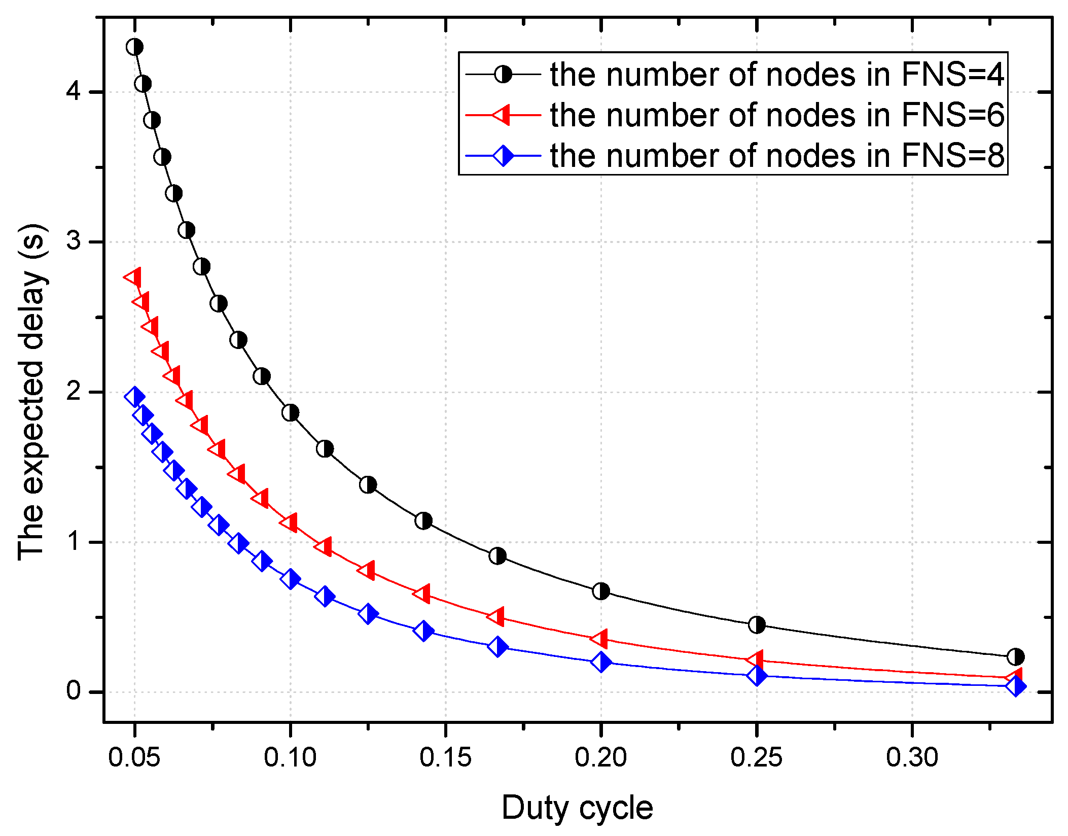
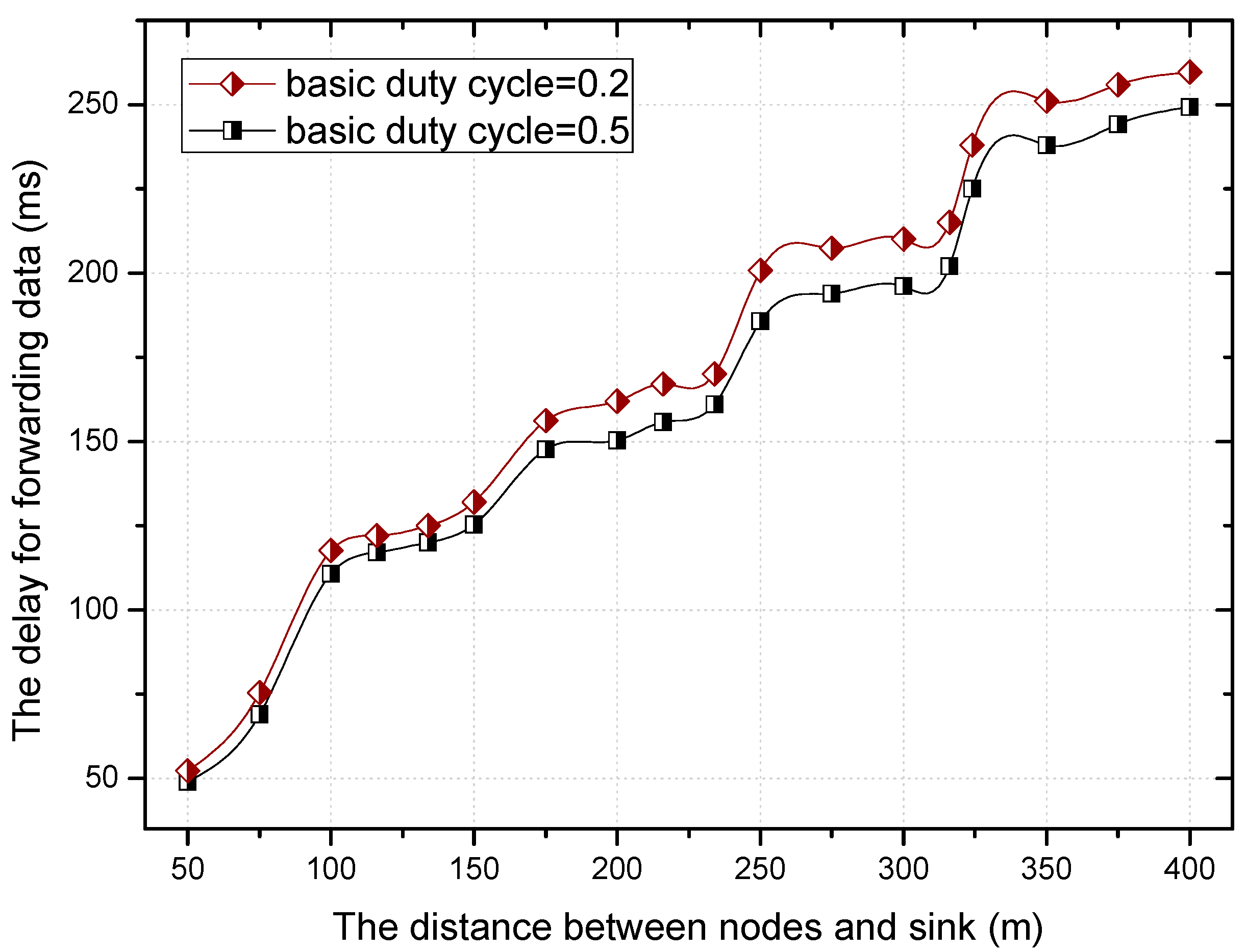
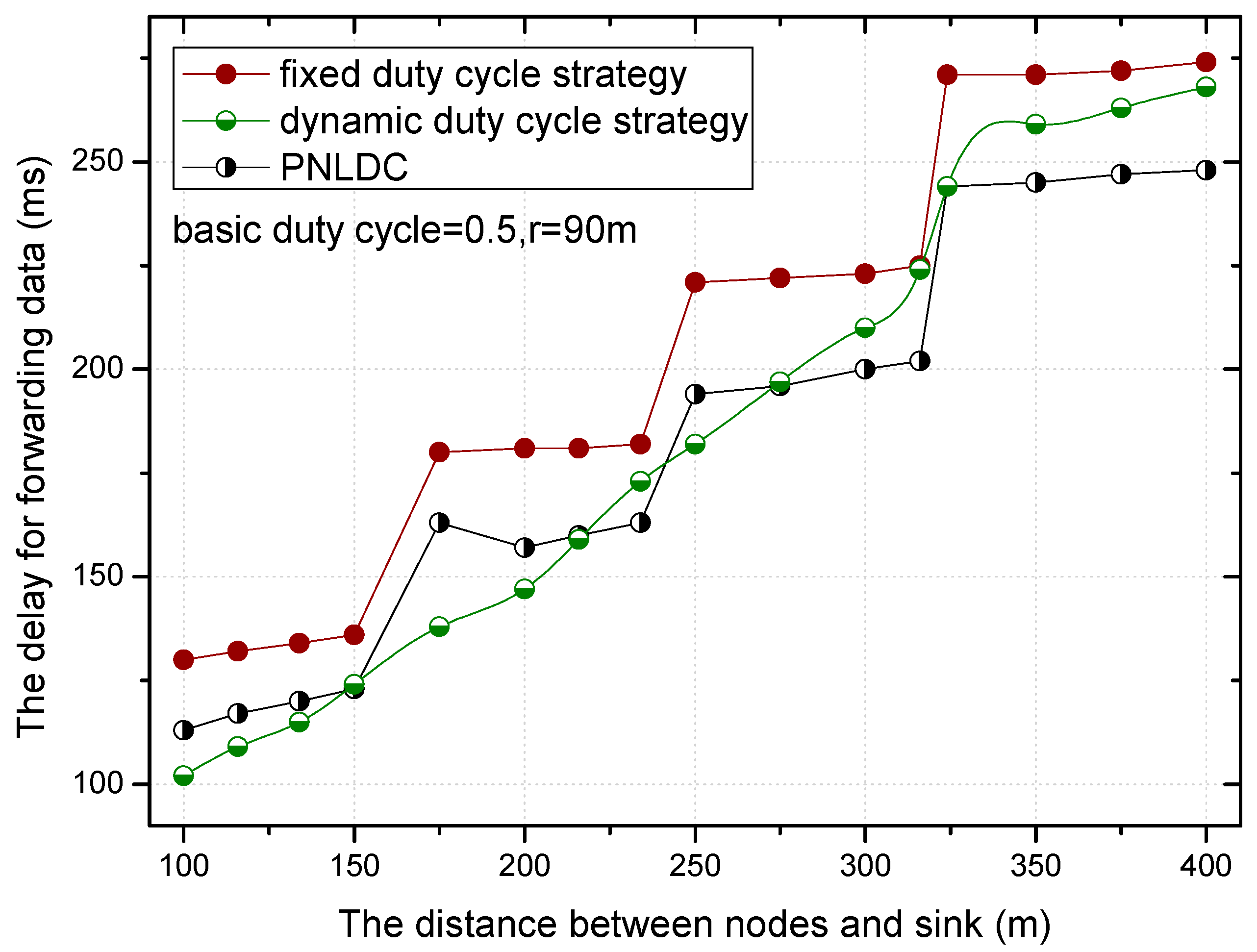
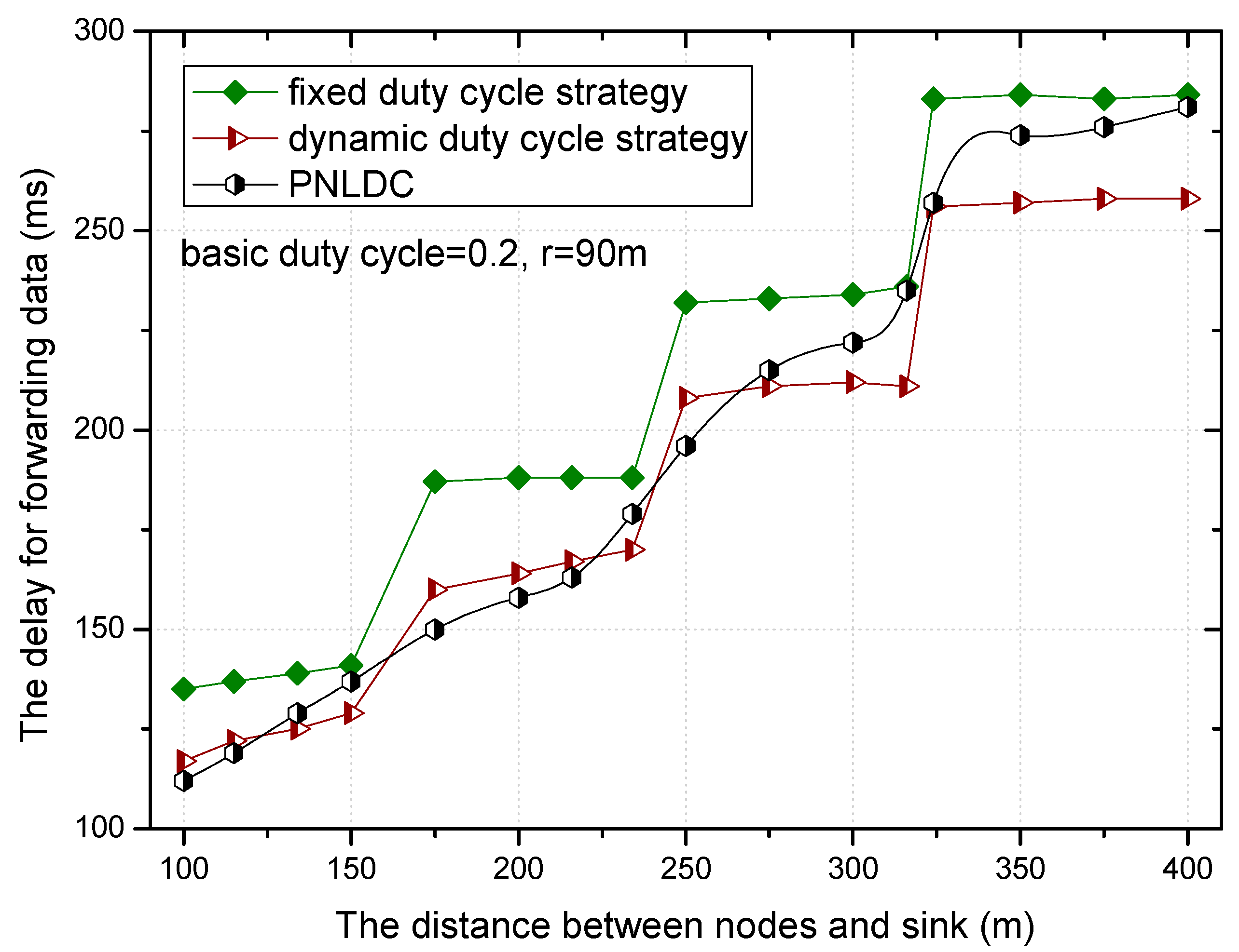
5.2. Delay of Forwarding Data
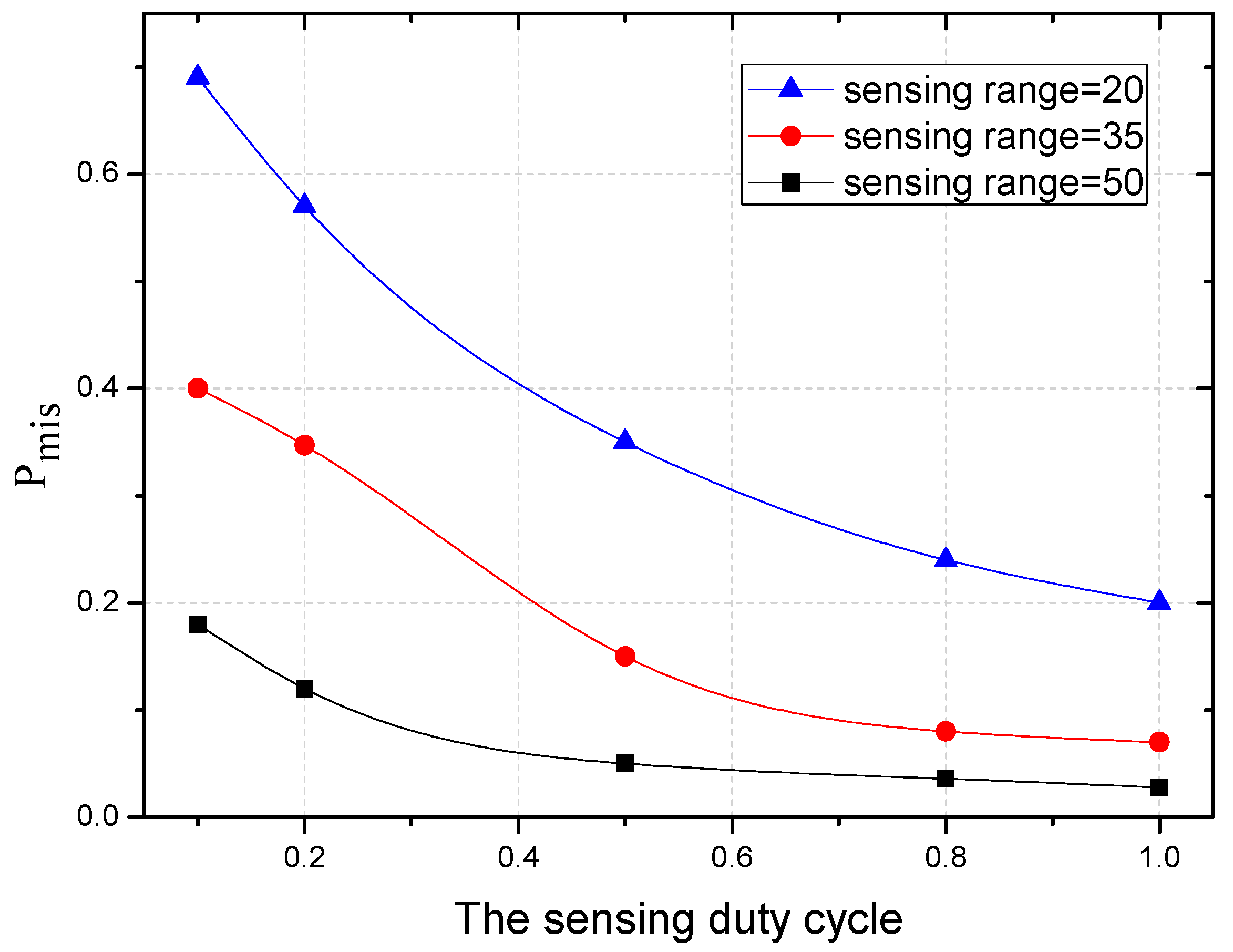
5.3. Delay for Detection
6. Conclusions and Future Work
Author Contributions
Funding
Conflicts of Interest
References
- Bhuiyan, M.Z.A.; Wu, J.; Wang, G.; Wang, T.; Hassan, M.M. e-Sampling: Event-Sensitive Autonomous Adaptive Sensing and Low-Cost Monitoring in Networked Sensing Systems. ACM Trans. Auton. Adapt. Syst. 2017, 12, 1. [Google Scholar] [CrossRef]
- Li, Z.; Chang, B.; Wang, S.; Liu, A.; Zeng, F.; Luo, G. Dynamic Compressive Wide-band Spectrum Sensing Based on Channel Energy Reconstruction in Cognitive Internet of Things. IEEE Trans. Ind. Inform. 2018, 1. [Google Scholar] [CrossRef]
- Ota, K.; Dong, M.; Gui, J.; Liu, A. QUOIN: Incentive Mechanisms for Crowd Sensing Networks. IEEE Netw. Mag. 2018, 32, 114–119. [Google Scholar] [CrossRef]
- Huang, M.; Liu, A.; Zhao, M.; Wang, T. Multi Working Sets Alternate Covering Scheme for Continuous Partial Coverage in WSNs. Peer Peer Netw. Appl. 2018. [Google Scholar] [CrossRef]
- Gui, J.S.; Hui, L.H.; Xiong, N.X. Enhancing Cellular Coverage Quality by Virtual Access Point and Wireless Power Transfer. Wirel. Commun. Mob. Comput. 2018, 2018, 9218239. [Google Scholar] [CrossRef]
- Jiang, W.; Wang, G.; Bhuiyan, M.Z.A.; Wu, J. Understanding graph-based trust evaluation in online social networks: Methodologies and challenges. ACM Comput. Surv. 2016, 49, 10. [Google Scholar] [CrossRef]
- Xu, Q.; Su, Z.; Zheng, Q.; Luo, M.; Dong, B. Secure Content Delivery with Edge Nodes to Save Caching Resources for Mobile Users in Green Cities. IEEE Trans. Ind. Inform. 2017, 1. [Google Scholar] [CrossRef]
- Yang, G.; He, S.; Shi, Z. Leveraging crowdsourcing for efficient malicious users detection in large-scale social networks. IEEE Internet Things J. 2017, 4, 330–339. [Google Scholar] [CrossRef]
- Bhuiyan, M.Z.A.; Wang, G.; Wu, J.; Cao, J.; Liu, X.; Wang, T. Dependable structural health monitoring using wireless sensor networks. IEEE Trans. Dependable Secur. Comput. 2017, 14, 363–376. [Google Scholar] [CrossRef]
- Xu, J.; Liu, A.; Xiong, N.; Wang, T.; Zuo, Z. Integrated Collaborative Filtering Recommendation in Social Cyber-Physical Systems. Int. J. Distrib. Sens. Netw. 2017, 13, 1550147717749745. [Google Scholar] [CrossRef]
- Liu, Y.; Liu, A.; Guo, S.; Li, Z.; Choi, Y.J. Context-aware collect data with energy efficient in Cyber-physical cloud systems. Futur. Gener. Comput. Syst. 2017. [Google Scholar] [CrossRef]
- Liu, X.; Xiong, N.; Zhang, N.; Liu, A.; Shen, H.; Huang, C. A Trust with Abstract Information Verified Routing Scheme for Cyber-physical Network. IEEE Access 2018, 6, 3882–3898. [Google Scholar] [CrossRef]
- Teng, H.; Liu, X.; Liu, A.; Shen, H.; Huang, C.; Wang, T. Adaptive transmission power control for reliable data forwarding in sensor based networks. Wirel. Commun. Mob. Comput. 2018, 2018, 2068375. [Google Scholar] [CrossRef]
- Liu, X.; Dong, M.; Liu, Y.; Liu, A.; Xiong, N. Construction Low Complexity and Low Delay CDS for Big Data Codes Dissemination. Complexity 2018, 2018, 5429546. [Google Scholar] [CrossRef]
- Sarkar, S.; Chatterjee, S.; Misra, S. Assessment of the Suitability of Fog Computing in the Context of Internet of Things. IEEE Trans. Cloud Comput. 2018, 6, 46–59. [Google Scholar] [CrossRef]
- Internet of Things Market Forecast: Cisco. Available online: http://postscapes.com/internet-of-things-market-size (accessed on 2 March 2018).
- Liu, X.; Zhao, S.; Liu, A.; Xiong, N.; Vasilakos, A.V. Knowledge-aware Proactive Nodes Selection Approach for Energy management in Internet of Things. Futur. Gener. Comput. Syst. 2017. [Google Scholar] [CrossRef]
- Wang, T.; Zhou, J.; Huang, M.; Bhuiyan, M.Z.A.; Liu, A.; Xu, W.; Xie, M. Fog-based Storage Technology to Fight with Cyber Threat. Futur. Gener. Comput. Syst. 2018, 83, 208–218. [Google Scholar] [CrossRef]
- Chen, X.; Pu, L.; Gao, L.; Wu, W.; Wu, D. Exploiting massive D2D collaboration for energy-efficient mobile edge computing. IEEE Wirel. Commun. 2017, 24, 64–71. [Google Scholar] [CrossRef]
- Misra, S.; Chatterjee, S.; Obaidat, M.S. On theoretical modeling of sensor cloud: A paradigm shift from wireless sensor network. IEEE Syst. J. 2017, 11, 1084–1093. [Google Scholar] [CrossRef]
- Li, J.; Li, Y.K.; Chen, X.; Lee, P.P.C.; Lou, W. A hybrid cloud approach for secure authorized deduplication. IEEE Trans. Parallel Distrib. Syst. 2015, 26, 1206–1216. [Google Scholar] [CrossRef]
- Li, J.; Li, J.; Chen, X.; Jia, C.; Lou, W. Identity-based encryption with outsourced revocation in cloud computing. IEEE Trans. Comput. 2015, 64, 425–437. [Google Scholar] [CrossRef]
- Åkerberg, J.; Gidlund, M.; Björkman, M. Future research challenges in wireless sensor and actuator networks targeting industrial automation. In Proceedings of the 9th IEEE International Conference on Industrial Informatics (INDIN), Lisbon, Portugal, 26–29 July 2011; Volume 9, pp. 410–415. [Google Scholar]
- Liu, A.; Huang, M.; Zhao, M.; Wang, T. A Smart High-Speed Backbone Path Construction Approach for Energy and Delay Optimization in WSNs. IEEE Access 2018, 6, 13836–13854. [Google Scholar] [CrossRef]
- Xie, K.; Wang, X.; Wen, J.; Cao, J. Cooperative routing with relay assignment in multiradio multihop wireless networks. IEEE/ACM Trans. Netw. 2016, 24, 859–872. [Google Scholar] [CrossRef]
- Li, X.; Liu, A.; Xie, M.; Xiong, N.; Zeng, Z.; Cai, Z. Adaptive Aggregation Routing to Reduce Delay for Multi-Layer Wireless Sensor Networks. Sensors 2018, 18, 1216. [Google Scholar] [CrossRef] [PubMed]
- Liu, A.; Zhao, S. High performance target tracking scheme with low prediction precision requirement in WSNs. Int. J. Ad Hoc Ubiquitous Comput. 2017. Available online: http://www.inderscience.com /info/ingeneral/forthcoming.php?jcode=ijahuc (accessed on 8 January 2018 ).
- Xiao, F.; Liu, W.; Li, Z.; Chen, L.; Wang, R. Noise-tolerant Wireless Sensor Networks Localization via Multi-norms Regularized Matrix Completion. IEEE Trans. Veh. Technol. 2018, 67, 2409–2419. [Google Scholar] [CrossRef]
- Song, J.; Han, S.; Mok, A.; Chen, D.; Lucas, M.; Nixon, M.; Pratt, W. WirelessHART: Applying wireless technology in real-time industrial process control. In Proceedings of the IEEE Real-Time and Embedded Technology and Applications Symposium, St. Louis, MO, USA, 22–24 April 2008; pp. 377–386. [Google Scholar]
- Deng, Q.; Li, X.; Li, Z.; Liu, A.; Choi, Y.-J. Electricity Cost Minimization for Delay-tolerant Basestation Powered by Heterogeneous Energy Source. KSII Trans. Internet Inf. Syst. 2017, 11, 5712–5728. [Google Scholar]
- Liu, Y.; Ota, K.; Zhang, K.; Ma, M.; Xiong, N.; Liu, A.; Long, J. QTSAC: A Energy efficient MAC Protocol for Delay Minimized in Wireless Sensor networks. IEEE Access 2018, 6, 8273–8291. [Google Scholar] [CrossRef]
- Liu, X.; Liu, Y.; Xiong, N.; Zhang, N.; Liu, A.; Shen, H.; Huang, C. Construction of Large-scale Low Cost Deliver Infrastructure using Vehicular Networks. IEEE Access 2018. [Google Scholar] [CrossRef]
- Dai, H.; Chen, G.; Wang, C.; Wang, S.; Wu, X.; Wu, F. Quality of energy provisioning for wireless power transfer. IEEE Trans. Parallel Distrib. Syst. 2015, 26, 527–537. [Google Scholar] [CrossRef]
- Zhou, K.; Gui, J.; Xiong, N. Improving cellular downlink throughput by multi-hop relay-assisted outband D2D communications. EURASIP J. Wirel. Commun. Netw. 2017, 2017, 209. [Google Scholar] [CrossRef]
- Xin, H.; Liu, X. Energy-balanced transmission with accurate distances for strip-based wireless sensor networks. IEEE Access 2017, 5, 16193–16204. [Google Scholar] [CrossRef]
- Liu, A.; Chen, W.; Liu, X. Delay Optimal Opportunistic Pipeline Routing Scheme for Cognitive Radio Sensor Networks. Int. J. Distrib. Sens. Netw. 2018, 14, 1550147718772532. [Google Scholar] [CrossRef]
- Chen, X.; Li, J.; Weng, J.; Ma, J.; Lou, W. Verifiable computation over large database with incremental updates. IEEE Trans. Comput. 2016, 65, 3184–3195. [Google Scholar] [CrossRef]
- Xie, G.; Ota, K.; Dong, M.; Pan, F.; Liu, A. Energy-efficient routing for mobile data collectors in wireless sensor networks with obstacles. Peer Peer Netw. Appl. 2017, 10, 472–483. [Google Scholar] [CrossRef]
- Liu, Q.; Liu, A. On the hybrid using of unicast-broadcast in wireless sensor networks. Comput. Electr. Eng. 2017. [Google Scholar] [CrossRef]
- Liu, X.; Li, G.; Zhang, S.; Liu, A. Big Program Code Dissemination Scheme for Emergency Software-define Wireless Sensor Networks. Peer Peer Netw. Appl. 2017, 1–22. [Google Scholar] [CrossRef]
- Liu, Y.; Liu, A.; Li, Y.; Li, Z.; Choi, Y.J.; Sekiya, H.; Li, J. APMD: A fast data transmission protocol with reliability guarantee for pervasive sensing data communication. Pervasive Mob. Comput. 2017, 41, 413–435. [Google Scholar] [CrossRef]
- Naveen, K.P.; Anurag, K. Relay selection for geographical forwarding in sleep-wake cycling wireless sensor networks. IEEE Trans. Mob. Comput. 2013, 12, 475–488. [Google Scholar] [CrossRef]
- Liu, X. Node Deployment Based on Extra Path Creation for Wireless Sensor Networks on Mountain Roads. IEEE Commun. Lett. 2017, 21, 2376–2379. [Google Scholar] [CrossRef]
- Cui, J.; Zhang, Y.; Cai, Z.; Liu, A.; Li, Y. Securing Display Path for Security-Sensitive Applications on Mobile Devices. CMC Comput. Mater. Contin. 2018, 55, 17–35. [Google Scholar]
- Han, S.; Lam, K.Y.; Chen, D.; Xiong, M.; Wang, J.; Ramamritham, K.; Mok, A.K. Online mode switch algorithms for maintaining data freshness in dynamic cyber-physical systems. IEEE Trans. Knowl. Data Eng. 2016, 28, 756–769. [Google Scholar] [CrossRef]
- Han, S.; Chen, D.; Xiong, M.; Lam, K.Y.; Mok, A.K.; Ramamritham, K. Schedulability analysis of deferrablescheduling algorithms for maintainingreal-time data freshness. IEEE Trans. Comput. 2014, 63, 979–994. [Google Scholar] [CrossRef]
- Song, J.; Mok, A.K.; Chen, D.; Nixon, M.; Blevins, T.; Wojsznis, W. Improving PID control with unreliable communications. In Proceedings of the ISA EXPO Technical Conference, Houston, TX, USA, 17–19 October 2006. [Google Scholar]
- Yu, K.; Gidlund, M.; Åkerberg, J.; Björkman, M. Performance evaluations and measurements of the REALFLOW routing protocol in wireless industrial networks. IEEE Trans. Ind. Inform. 2017, 13, 1410–1420. [Google Scholar] [CrossRef]
- Zheng, T.; Gidlund, M.; Åkerberg, J. WirArb: A new MAC protocol for time critical industrial wireless sensor network applications. IEEE Sens. J. 2016, 16, 2127–2139. [Google Scholar] [CrossRef]
- Hsu, T.H.; Kim, T.H.; Chen, C.C.; Wu, J.S. A dynamic traffic-aware duty cycle adjustment MAC protocol for energy conserving in wireless sensor networks. Int. J. Distrib. Sens. Netw. 2012, 8, 790131. [Google Scholar] [CrossRef]
- Liu, Q.; Wang, G.; Liu, X.; Peng, T.; Wu, J. Achieving Reliable and Secure Services in Cloud Computing Environments. Comput. Electr. Eng. 2017, 59, 153–164. [Google Scholar] [CrossRef]
- Xie, K.; Cao, J.; Wang, X.; Wen, J. Optimal resource allocation for reliable and energy efficient cooperative communications. IEEE Trans. Wirel. Commun. 2013, 12, 4994–5007. [Google Scholar] [CrossRef]
- Zhang, N.; Liang, H.; Cheng, N.; Tang, Y.; Mark, J.W.; Shen, X.S. Dynamic spectrum access in multi-channel cognitive radio networks. IEEE J. Sel. Areas Commun. 2014, 32, 2053–2064. [Google Scholar] [CrossRef]
- Zhang, N.; Cheng, N.; Lu, N.; Zhou, H.; Mark, J.W.; Shen, X. Risk-aware cooperative spectrum access for multi-channel cognitive radio networks. IEEE J. Sel. Areas Commun. 2014, 32, 516–527. [Google Scholar] [CrossRef]
- Dhanalakshmi, R.; Vadivel, A.; Parthiban, P. Shortest Path Routing in Solar Powered WSNs Using Soft Computing Techniques. J. Sci. Ind. Res. 2017, 76, 23–27. [Google Scholar]
- Tang, J.; Liu, A.; Zhang, J.; Zeng, Z.; Xiong, N.; Wang, T. A Security Routing Scheme Using Traceback Approach for Energy Harvesting Sensor Networks. Sensors 2018, 18, 751. [Google Scholar] [CrossRef] [PubMed]
- Li, J.; Chen, X.; Huang, X.; Tang, S.; Xiang, Y.; Hassan, M.M.; Alelaiwi, A. Secure distributed deduplication systems with improved reliability. IEEE Trans. Comput. 2015, 64, 3569–3579. [Google Scholar] [CrossRef]
- Gui, J.; Deng, J. Multi-hop Relay-Aided Underlay D2D Communications for Improving Cellular Coverage Quality. IEEE Access 2018, 6, 14318–14338. [Google Scholar] [CrossRef]
- Salehi, M.; Boukerche, A. A novel packet salvaging model to improve the security of opportunistic routing protocols. Comput. Netw. 2017, 122, 163–178. [Google Scholar] [CrossRef]
- Joo, C.; Shroff, N.B. On the delay performance of in-network aggregation in lossy wireless sensor networks. IEEE/ACM Trans. Netw. 2014, 22, 662–673. [Google Scholar] [CrossRef]
- Liu, Y.; Liu, A.; Hu, Y.; Li, Z.; Choi, Y.J.; Sekiya, H.; Li, J. FFSC: An energy efficiency communications approach for delay minimizing in internet of things. IEEE Access 2016, 4, 3775–3793. [Google Scholar] [CrossRef]
- Guo, Y.; Liu, F.; Cai, Z.; Xiao, N.; Zhao, Z. Edge-Based Efficient Search over Encrypted Data Mobile Cloud Storage. Sensors 2018, 18, 1189. [Google Scholar] [CrossRef] [PubMed]
- Xu, X.; Yuan, M.; Liu, X.; Liu, A.; Xiong, N.; Cai, Z.; Wang, T. Cross-layer Optimized Opportunistic Routing Scheme for Loss-and-delay Sensitive WSNs. Sensors 2018, 18, 1713. [Google Scholar] [CrossRef]
- Huang, M.; Liu, Y.; Zhang, N.; Xiong, N.; Liu, A.; Zeng, Z.; Song, H. A Services Routing based Caching Scheme for Cloud Assisted CRNs. IEEE Access 2018, 6, 15787–15805. [Google Scholar] [CrossRef]
- Hu, Y.; Liu, A. Improving the quality of mobile target detection through portion of node with fully duty cycle in WSNs. Comput. Syst. Sci. Eng. 2016, 31, 5–17. [Google Scholar]
- Medagliani, P.; Leguay, J.; Ferrari, G.; Gay, V.; Lopez-Ramos, M. Energy-efficient mobile target detection in wireless sensor networks with random node deployment and partial coverage. Pervasive Mob. Comput. 2012, 8, 429–447. [Google Scholar] [CrossRef]


| Parameter | Description | Value |
|---|---|---|
| Initial energy | 0.5 J | |
| Communication duration | 100 ms | |
| Power consumed by transmission | 0.0511 W | |
| Power consumed by reception | 0.0588 W | |
| Power consumed by sleeping | 2.4 × 10⁻⁷ W | |
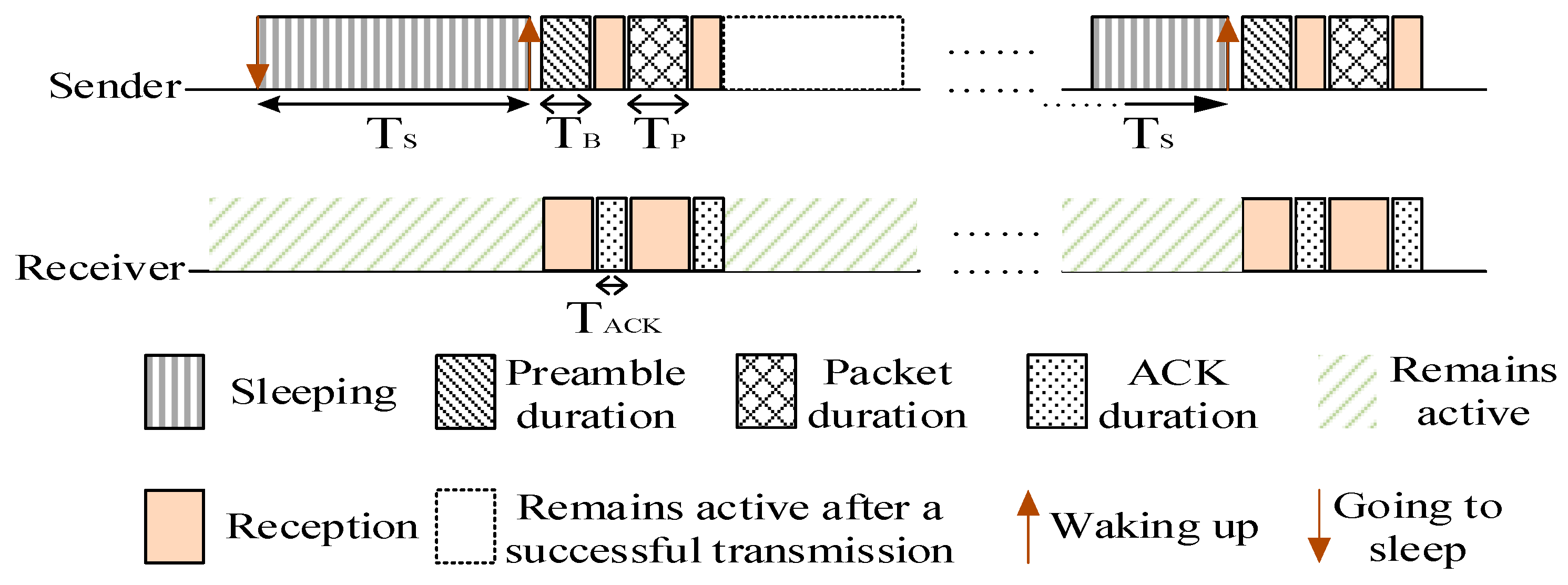
| Preamble duration | 0.26 ms | |
| Acknowledge window duration | 0.26 ms | |
| Packet duration | 0.93 ms | |
| Sensing duration | 15 s |
© 2018 by the authors. Licensee MDPI, Basel, Switzerland. This article is an open access article distributed under the terms and conditions of the Creative Commons Attribution (CC BY) license (http://creativecommons.org/licenses/by/4.0/).
Share and Cite
Wu, M.; Wu, Y.; Liu, C.; Cai, Z.; Xiong, N.N.; Liu, A.; Ma, M. An Effective Delay Reduction Approach through a Portion of Nodes with a Larger Duty Cycle for Industrial WSNs. Sensors 2018, 18, 1535. https://doi.org/10.3390/s18051535
Wu M, Wu Y, Liu C, Cai Z, Xiong NN, Liu A, Ma M. An Effective Delay Reduction Approach through a Portion of Nodes with a Larger Duty Cycle for Industrial WSNs. Sensors. 2018; 18(5):1535. https://doi.org/10.3390/s18051535
Chicago/Turabian StyleWu, Minrui, Yanhui Wu, Chuyao Liu, Zhiping Cai, Neal N. Xiong, Anfeng Liu, and Ming Ma. 2018. "An Effective Delay Reduction Approach through a Portion of Nodes with a Larger Duty Cycle for Industrial WSNs" Sensors 18, no. 5: 1535. https://doi.org/10.3390/s18051535
APA StyleWu, M., Wu, Y., Liu, C., Cai, Z., Xiong, N. N., Liu, A., & Ma, M. (2018). An Effective Delay Reduction Approach through a Portion of Nodes with a Larger Duty Cycle for Industrial WSNs. Sensors, 18(5), 1535. https://doi.org/10.3390/s18051535