Abstract
This paper proposes a novel filtering design, from a viewpoint of identification instead of the conventional nonlinear estimation schemes (NESs), to improve the performance of orbit state estimation for a space target. First, a nonlinear perturbation is viewed or modeled as an unknown input (UI) coupled with the orbit state, to avoid the intractable nonlinear perturbation integral (INPI) required by NESs. Then, a simultaneous mean and covariance correction filter (SMCCF), based on a two-stage expectation maximization (EM) framework, is proposed to simply and analytically fit or identify the first two moments (FTM) of the perturbation (viewed as UI), instead of directly computing such the INPI in NESs. Orbit estimation performance is greatly improved by utilizing the fit UI-FTM to simultaneously correct the state estimation and its covariance. Third, depending on whether enough information is mined, SMCCF should outperform existing NESs or the standard identification algorithms (which view the UI as a constant independent of the state and only utilize the identified UI-mean to correct the state estimation, regardless of its covariance), since it further incorporates the useful covariance information in addition to the mean of the UI. Finally, our simulations demonstrate the superior performance of SMCCF via an orbit estimation example.
1. Introduction
The orbit estimation problem is to obtain an accurate estimation of a space target’s (e.g., satellite) position and velocity from noisy observations. The dynamic model of a space target is given below by considering perturbations [1]:
where is the position of the space target in the inertial coordinate frame (I-J-K), , w is the white Gaussian noise process, and is the instantaneous acceleration due to the perturbation [2]. is the dimensionless second zonal harmonic that quantifies the major oblateness effect of the Earth. Specially, the perturbation may cause a noticeable precession of low-earth orbit (LEO) satellites, and makes the orbital dynamics model to be a strongly nonlinear function. Thus, solving the orbit estimation problem essentially depends on designing a kind of nonlinear state estimation schemes.
At present, nonlinear estimation schemes (NESs) are generally developed from a Bayesian inference framework (BIF) [3] and employed as the widely accepted methods for estimating the space target orbital state. The BIF framework structure is given in Figure 1.
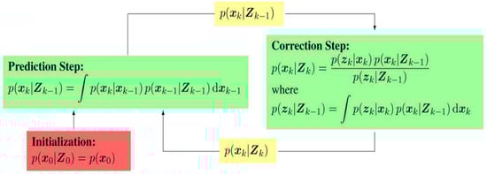
Figure 1.
Bayesian inference framework.
Obviously, to implement BIF in order to estimate the orbit state, NES requires one to compute the strongly nonlinear integral of the perturbation. As an example for Gaussian filters [4]:
where is assumed to be a Gaussian distribution, and denotes the sequence of measurements. The numerical computation of such an integral is both complicated and intractable, such that orbit estimation accuracy may be weak and cannot meet real-time performance requirements. For orbit tracking of a space target, a data-starved and uncertain state evolution [5] requires that the tracking algorithm should be rapid and high-precision.
- Here, data-starved does not mean a lack of measurements. Rather, it implies that due to the large number of space objectives, the collection, association, processing, and fusion of the measurements needs a lot of time. Hence, the measurement update rate and period are relatively elongated. This requires the tracking algorithm deals with data as efficiently and rapidly as possible.
- Under a data-starved environment or long data update period, as a result of the consistent long-term (usually several orbital periods) propagation of state uncertainties in high fidelity physics models between measurement updates, a state which is initially Gaussian will inevitably become significantly non-Gaussian or uncertain if propagated over a sufficiently long time span. This requires that the tracking algorithm should be accurate when estimating the uncertain or non-Gaussian state.
The traditional NES, based on BIF, does not meet the rapidity and high-precision requirements due to the complicated and intractable nonlinear perturbation integral.
In order to avoid the nonlinear perturbation integral computation, a joint estimation and identification scheme (JEIS) simply views as an additional unknown input (UI) and analytically identifies to accurately correct the orbit state estimation [6]. Such analytical identification in JEIS decreases the algorithm complexity while improving the orbit estimation accuracy to some degree by feedback correction. In other words, this paper mainly aims to transfer the intractable nonlinear perturbation integral issue into that of perturbation (viewed as UI) identification, to simplify the orbit estimation algorithm complexity and improve its accuracy.
As a classical representative of JEIS, the expectation maximization (EM) algorithm has received continuous attention and research. The EM framework fits in with the requirements of JESI, as shown in Figure 2. However, the existing EM algorithms always model the UI as a constant variable, independent of the state [6], and only identify the mean of the UI. In the perturbation, (viewed as UI in JEIS) depends on the state, so it requires at least the first two moments (FTM), i.e., the mean and covariance. To further improve the accuracy of orbit estimation, it is important to research the novel EM algorithm; to identify the UI-FTM (i.e., perturbation-FTM) which simultaneously corrects the state estimation and its covariance. Unfortunately, the existing EM is incapable of dealing with the case when the UI is associated with the state.
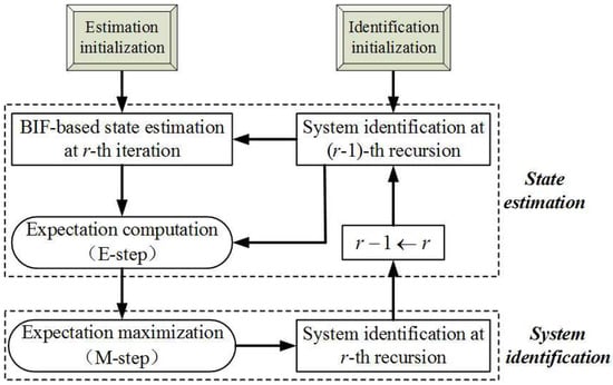
Figure 2.
Schematic of the expectation maximization (EM) algorithm, where BIF refers to the Bayesian inference framework.
Following this idea, that the original orbit estimation is transferred into JESI, we design a novel two-stage EM algorithm (Figure 3 and Figure 4) to deal with the key difficulty of how to simultaneously fit or identify the FTM of UI associated with the state. The main contributions are that: (1) The first EM executes joint orbit state estimation and pseudo measurement (PM) identification using networked multi-sensor observations. PMs can be understood as the indirect reflection of UI from the real observed measurements. (2) The second EM is designed for fitting the UI-FTM by UI-PMs from different sensors, and then used to simultaneously correct the orbit state estimation and its covariance in the first EM. Finally, (3) the identification and fitting computations in these two EMs are analytical, which contributes to rapid and efficient implementation. The simultaneous correction of UI-FTM to the state estimate, as shown in Figure 3, improves the orbit state estimation accuracy. By doing this, a novel simultaneous mean and covariance correction filter (SMCCF) is proposed and achieved. Indeed, vastly different from the standard EM-based filtering scheme, which only estimates the mean characteristic of UI, the novel SMCCF scheme further determines the covariance characteristic of UI. In other words, the joint properties (i.e., both mean and covariance) characterizing the UI in the new scheme provide richer information compared to the single one (i.e., only mean) of the standard approach, which contributes to improved state estimation.
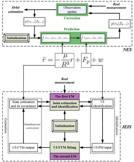
Figure 3.
Two-stage EM algorithm.
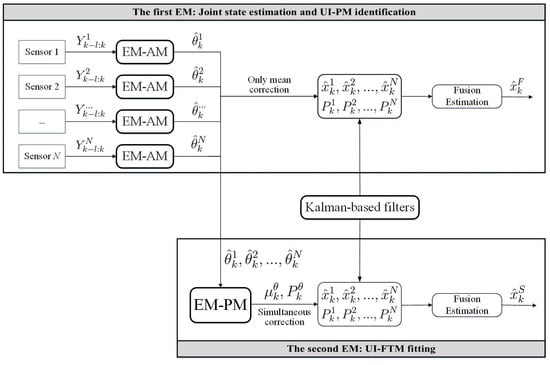
Figure 4.
The basic building blocks of the simultaneous mean and covariance correction filter (SMCCF).
In this paper, the first EM is called the EM-AM since from the signal input viewpoint it mines the actual measurements (AMs) to characterize the UI, as shown in Figure 3. Similarly, we call the second EM as the EM-PM since it utilizes the PM as input to further fit the UI-FTM. However, different from Reference [7], the expanded contributions of this paper lie in that: (1) we specifically define the pseudo measurement and explain its physical implication (see the test following Equation(19)); (2) initialization of EM-AM plays a key role on the SMCCF performance, so we refine initialization of the EM-AM by using a relatively simple forward–backward smoother, instead of the previous two-filters (see Figure 5 and Figure 6, and Remarks 2 and 3); (3) we elaborate the relationship between EM-AM and EM-PM (see Figure 7 and Figure 8), and the algorithm execution program of SMCCF (see Figure 9 in Section V-A), in order to facilitate application of SMCCF in practical engineering; and (4) the performance of SMCCF is thoroughly demonstrated by a space target orbit estimation problem and compared to the present classical methods (see Section VI-B). Also different from other EM-based UI identification issues, for example Reference [6], which are only concerned with the mean of UI, this paper designs the novel SMCCF which simultaneously fits the UI-FTM.
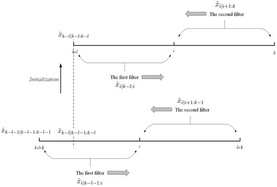
Figure 5.
The two-filter smoother and its initialization in EM-AM.
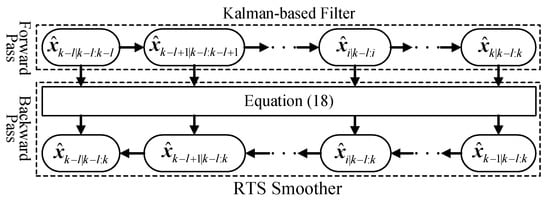
Figure 6.
The forward-backward smoother.
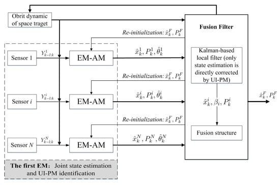
Figure 7.
Direct estimation fusion from EM-AM.
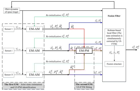
Figure 8.
SMCCF.
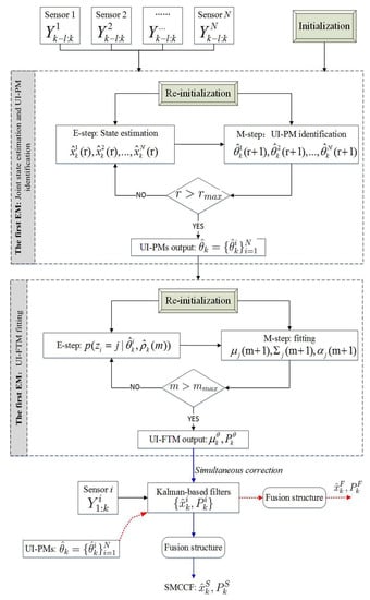
Figure 9.
SMCCF execution program.
This paper is organized as follows. Section 2 formulates the problem. Section 3 and Section 4 design the first and second EMs in the two-stage EM algorithm, respectively. Section 5 gives the fusion structure for combining the two EMs and achieving SMCCF. Section 6 demonstrates the superiority of SMCCF to the standard NES, including the extended Kalman filter (EKF) and the cubature Kalman filter (CKF), by an elaborate simulation of a space target orbit estimation. Finally, some conclusions are drawn in Section 7, including the future work.
Notations. The superscripts -1 and represent the inverse and transpose operations of a matrix, respectively. If X is a positive semi-definite or positive definite matrix, we simply write or . denotes the variable x obey a Gaussian distribution with mean and covariance . is the probability, for example describes the conditional probability of the variable A on B. and represent the expectation or conditional expectation, respectively. We define two operations and . The symbols and on top of a random variable, represent an estimate and its error, respectively. For example, denotes the estimate of variable x and its estimation error is . denotes the trace of matrix.
2. Problem Formulation
Consider a general discrete-time stochastic system with additive UIs in the dynamic and measurement models:
where represent the state and measurement vectors, and are the known dynamic and measurement functions, respectively. The matrices , and are known. and are uncorrelated, zero-mean Gaussian white noise terms satisfying and , where is the Kronecker delta function. The initial state is a Gaussian vector with mean and covariance . Here, , and are mutually independent. The parameters , and are unknown UIs which are associated with the state. Also, we set .
Remark 1.
The model in Equation (1) is common in practical engineering. Consider the example of space object tracking, whose dynamic model is formulated as follows:
The last term in Equation (2) is known as the perturbation, , which is obviously associated with the state. If we regard the perturbation as UI, space object tracking can be modeled by Equation (1). Another example is tracking a maneuvering non-cooperative target, whose dynamic model, due to the modeling error, can be represented by:
If is considered as the UI, which is obviously coupled with the state, we can also formulate maneuvering target tracking in terms of the model in Equation (1).
Due to the characteristic that the UI is highly coupled with the system state, possesses the FTM. In this case, if we only consider the UI’s mean to correct the state, the estimation accuracy may be undesirable. A feasible method to improve the accuracy is to correct the state by using both the UI-FTM simultaneously. Hence, our objective is to not only identify the mean but also to fit the covariance of the UI. Unfortunately, the existing methods, such as JESI or the standard EM, always regard the UI as a constant. So they all ignore the covariance property of UI, which limits to solving the state estimation problem corresponding to Equation (1).
Combining Equations (1) and (2), we view the perturbation in space target orbit estimation or in tracking as a UI associated with the state. Our aim is to explore the novel EM algorithm for fitting the UI-FTM based on the actual measurements (AMs) from multi-sensors, where l represents the sliding window length. Furthermore, the orbit state estimation is simultaneously corrected by using the fitted UI-FTM.
Different from the classical EM algorithm in Reference [6], a two-stage EM scheme is proposed, as shown in Figure 4 which is a further refinement of Figure 3. In the first stage, for each sensor with , EM carries out joint state estimation and UI-PM identification, where PM refers to pseudo measurement. N sensors need N EMs, which run in parallel. All EMs output two groups; the state estimation and the UI-PM identification , where corresponds to the i-th sensor or the i-th EM. Indeed, the EM in the first stage reflects or characterizes UI by the output PM from the input AM. Thus, we also call the first EM as EM-AM, from a signal input viewpoint. The state estimation in EM-AM running process is only corrected by the PM . In the second stage, we further fit the UI-PM by a Gaussian mixture distribution with mean and covariance , which can be fed back into the first EM to jointly correct the state estimation and its covariance. Similarly, we name the second EM as EM-PM. By linking these two EMs, the SMCCF is proposed by designing the fusion structure. From a sense of whether enough information is mined or utilized, the by SMCCF should be superior to the by the existing nonlinear filters or algorithms in accuracy, since the former further mines covariance information in addition to the mean of UI.
3. EM-AM
The EM algorithm was introduced by Dempster et al. [8] to solve maximum likelihood (ML) estimation with incomplete or missing data. If we consider the state in Equation (1) as the missing data and as the parameters which need to be identified, then the EM framework [9] is suitable for joint state estimation and UI-PM identification precisely.
To implement the EM-AM algorithm in each sensor in Figure 4, we first need to compute the conditional expectation, , of the complete data log-likelihood function in the E-step. Before addressing this, by first using Bayes’ rule and the Markov property of the model in Equation (1), we have:
Then, applying the following Gaussian approximation:
Equation (4) can be rearranged to yield:
where is a constant independent of , and is thus omitted, and:
The following subsections outline the steps to achieve EM-AM according to Figure 2; the E-step and M-step.
3.1. E-Step in EM-AM
Taking the expectation of Equation (7) with respect to the probability density function , we can obtain:
where is a constant corresponding to . Note that this posterior probability, , corresponds to the state estimation on knowing the identification value at the r-th iteration of EM-AM. It can be computed by Kalman-based estimators, such as Gaussian filters including EKF, and CKF, among others. Thus, we have:
where the computations of Equations (13) and (14) refer to:
and and are the posterior estimates of the state under the measurements from the interval [, k] with the minimum mean square error (MMSE) criterion:
In Equations (8) and (12), the terms and are associated with the UI , but is hidden in the probability . Hence, we can not obtain the dominant expressions of and like we can for , , , and . In order to compute the dominant derivative of with respect to , we have to ignore and . But ignoring and is reasonable in some sense, because: (1) if , then equals , which is independent of , and (2) since the UI is associated with the state in our problem, is time-varying. In order to quickly reflect or sketch this time-varying UI, it should gradually forget the previous information while preserving the current information in a sliding window of length l. This means that the previous measurements in interval are given up.
In order to compute , the state estimation and its covariance in the interval must be computed first, which is known as a smooth problem and can be implemented by using a fixed interval smoother. One example is the two-filter smoother [10], which is formulated as follows:
where, as shown in Figure 5 the first filter (i.e., , ) is computed by Kalman-based filtering under the model in Equation (1) and the second filter (i.e., , ) is also computed with a similar Kalman-based filter but under the inverse form of Equation (1), which runs backwards in time. The unscented Kalman filter (UKS) presented in Reference [11] can be understood as an approximate implementation of this form of smoother in nonlinear systems.
Another type of smoother is the forward-backward smoother [12], names as Rauch-Tung-Striebel (RTS) Smoother:
Here, the forward pass applies Kalman-based filters to compute the filtering estimates , and the predictive estimates , , which are same as those in two-filter smoother. But in the backward pass, the smoothing recursion starts from last time step k and proceeds backwards in time. That is, to compute the smoothing estimation from , to , , which is different from the second filter in the two-filter smoother. A derivation of the structure in Equation (18), can be found in References [13,14,15], and its computation program is shown in Figure 6.
Remark 2.
A key point of implementing Equation (17) is initialization. If we regard the interval as (where the initial value is ), the first filter in Equation (17) should be initialized by , which is obtained in the proposed SMCCF by knowing the identified UI-FTM in the interval . In more detail, the first filter is easily initialized by a standard Kalman-based filter with the initial state value . The initialization of the second filter depends on that of the first filter. In other words, the second filter also operates a standard Kalman-based filter but under the inverse form of Equation (1) with the initial value , which is obtained by the first filter. The details of the second filter are elaborated in Reference [11]. The inverse computation of Equation (1) complicates the two-filter smoother. Specifically for nonlinear systems, it is intractable and even infeasible to obtain the model’s inverse form.
Remark 3.
In the forward-backward smoother, only the forward filter needs to be initialized, which is similar to the initialization of the first filter in the two-filter smoother. While the backward smoothing computation in Equation (18) proceeds backwards in time, i.e., from to . Note that is obtained by the forward filter. Hence, from the viewpoint of a simpler initialization, the forward-backward smoother outperforms the two-filter one in operation. More importantly, the former contributes to simply achieving the following M-step in EM-AM, without computing the inverse form of the nonlinear model. Due to the above two reasons, this paper implements the forward-backward smoother for the state estimation in EM-AM.
3.2. M-Step in EM-AM
So far, we have completed the computation of the expectation with respect to by the E-step. Before maximizing , the pseudo measurement (PM) of UI is defined as follows:
where is coupled to the state, but the inherent coupling characteristic is unknown. Equation (19) indeed implies the posterior identification of UI under actual measurements, i.e., that affects the state estimation and further acts on the UI identification (). Hence PM’s definition concretely links estimation and identification in EM-AM.
The M-step requires a maximization of with respect to . Here, we let the first derivatives of with respect to to be zero directly:
Thus, we have:
where:
In other words, from Equation (20) to (23), PM can be understood as an average and indirect measurement of UIs by allowing actual observations to further influence UI-PM identification. The derivatives in Equations (20) and (21) essentially treat UIs (a and b) as kinds of average values in the interval . Thus UI-PM identification in Equations (22) and (23) indeed determines the estimated values and at the -th iteration:
Further, the second derivatives of with respect to :
are strictly negative-definite only if and , which can be always guaranteed in practice. This implies that Equations (22) and (23) uniquely maximize the convex . However, Equations (22) and (23) are only formally analytical and optimal since they need to approximately compute the following general integrals:
where generalizes the functions and , while describes or . As mentioned in Remark 3, if we use Kalman-based filters to compute such integrals, for example the Gaussian filter, denotes the corresponding Gaussian distribution. So numerical approximations such as EKF, and CKF can implement this integral computation (see References [16,17]). To avoid repetition, the process is omitted.
After identifying the UI-PM, how to further fit the UI-FTM with the PM will be dealt with in designing the EM-PM. According to Figure 4, every sensor runs one EM-AM to output a group of . In fact, only is directly corrected by UI-PM in the EM-AM. The following section designs the EM-PM for fitting the covariance of UI-PM to correct the estimation covariance .
Remark 4.
At each recursion, the PM parameter is initialized with the previous PM identification, i.e., with . At the beginning time, can be initialized by prior information. For example, is computed from and by performing one recursion of the conventional nonlinear filtering, i.e., through the perturbation nonlinear integral to compute :
whose implementation is similar to that in Equation (26).
4. EM-PM
This section will fit the UI-FTM from the identified UI-PM in the probability domain, not the time-domain, by the EM algorithm. The UI-FTM fitting issue is to find the available probability density for describing the stochastic property of UI-PM, , where corresponds to the i-th sensor. It has been proven that a Gaussian mixture (GM) form can approximate any probability density function as closely as desired [16]. In order to determine the underlying probability distribution of the identified UI-PM set, at time k, we assume that the stochastic property of UI-PM is generated using M probability distributions where each is a Gaussian function with weight , mean , and covariance :
where are the associated parameters with UI-FTM fitting, , M is the number of Gaussian components in the GM, and is a multi-dimensional Gaussian probability density. The UI-FTM fitting is further transferred into the parameter identification of .
A detailed discussion for GM fitting based on the EM framework has been proposed in Reference [19]. Here, we only give a brief derivation about how to apply EM for fitting UI-FTM. First, the log-likelihood function of can be written as:
where . Direct maximization of Equation (29) can not be achieved since we don’t know which Gaussian component in the GM is the most suitable for expressing or fitting the probability of the j-th UI-PM . For dealing with this key point, a missing variable is introduced, which establishes a simple relation between the UI-PM and Gaussian components. Elaborately, and denotes that the i-th PM, , is probably characterized by the j-th Gaussian component, i.e., . By doing this, constructs the complete-data set for further establishing the complete-data likelihood function:
where the subscript denotes all of the Gaussian components which the i-th PM, , may correspond to. Indeed:
with . It should be emphasized that and have a one-to-one correspondence, which well explains Equation (30).
Then, the E-step needs to evaluate the conditional expectation of under :
where is the fitting result of in the m-th iteration.
Application of the following equation:
to further arrange Equation (31) obtains:
with:
where d is the dimension of , denotes the estimated probability that the j-th Gaussian component matches the i-th PM, , under knowing , and and are the m-th identification values of weight and mean/covariance corresponding to the j-th Gaussian component.
In the M-step, by making the following first derivatives as zero:
the parameters of are re-estimated with the updated probabilities:
Identifying requires optimization of the following term of Equation (32):
with the constraint . However, direct optimization with respect to is difficult. For simplicity, we equivalently construct:
Thus, making the first derivative of Equation (40) with respect to zero, one obtains:
Finally, applying the following equation:
to rearrange Equation (41), gives the weight update:
Summarizing the above, the fit mean, , and covariance, , of the UI-PM set, , are obtained as follows:
which corresponds to the output of the EM-PM in Figure 4. Here, , , and are the terminatively optimized parameters serving for the j-th Gaussian component at time k.
Remark 5.
EM-PM is initialized by directly computing the stochastic characteristics (average and variance) of from multi-sensors in time-domain. Although it may be simple and obvious, such the initialization is in line with the stochastic essence. Moreover, the initialization has no effect on the terminative convergence of the EM-PM, since the convex optimization of Equations (36) and (37) uniquely maximize the expectation.
5. SMCCF
After achieving EM-AM and EM-PM, this section aims to link them and further clarify their input-output relationship with each other. Before doing this, as a comparison, we first show the execution program of directly using the state estimation from the EM-AM output in Figure 7 (as a refinement of the first EM in Figure 4). By using EKF to implement the state estimation computation in the EM-AM, we have:
- Prediction
- Updatewhere denotes the identified UI-PM by the EM-AM corresponding to the i-th sensor, and are the Jacobian matrices of the dynamic and measurement models. Obviously, in each EM-AM, only the state estimation is corrected by the UI-PM while its covariance computation is the same as that in standard Kalman-based filter. Besides EKF, one has a freedom to select other Kalman-based filters for implementing the state estimation in EM-AM, such as the above-mentioned nonlinear Gaussian filters including UKF, and CKF, among others.
After obtaining N groups of , we use the well-known Federal structure to directly fuse as follows:
where corresponding to Figure 7, the filter weight . Of course, there also exist other estimation fusion structures, which have been well studied at present. However, this paper mainly wishes to focus on demonstrating the feasibility and superiority of the simultaneous correction forms in the following (Equation (48)), as compared to the standard mean-based correction form in Equations (45) and (46). Thus, we choose the relatively simple Federal structure for trying to best eliminate the possible influence or interference of fusion on the proposed simultaneous correction here.
The following continues to combine the EM-AM and EM-PM as shown in Figure 8 (which is a refinement of Figure 4). Different from Figure 7, the SMCCF adds the EM-PM between the EM-AM and Federal fusion structures to fit the UI-FTM. Before carrying out fusion, the state estimation and its covariance are simultaneously corrected by the UI-FTM. This means that if the EM-PM fits and as given in Equations (43) and (44), then employing EKF again as an example, we have:
Again the above-mentioned Federal structure in Equation (47) is used to fuse the state estimation and achieve the SMCCF, denoted as and . In fact, Figure 7 is based on the standard filter structure in Equations (45) and (46) , where the UI-PM identification values are directly used for correcting the state prediction and the measurement prediction, regardless of their covariances. But Figure 8 is based on the SMCCF structure in Equation (48), where are further mined from by adding the second EM part to simultaneously correct the predictions and the corresponding covariances.
Remark 6.
Of course, there are other execution programs which link the EM-AM and EM-PM to achieve SMCCF. For example, at each iteration of the EM-AM, the output PM identifications by multi-sensors are fit by EM-PM, and fed back to simultaneously correct the state estimation and its covariance. But, this paper mainly aims to demonstrate the superiority of the novel JESI to the standard NES, and SMCCF to the standard nonlinear filters, including EKF, and UKF, among others. The performance analysis or comparison of different fusion structures will be explored in the future work.
Remark 7.
Maybe, one can find that the state estimation forms between Equations (17), (18), (45), (46), and (48), are slightly different from each other. At each time-recursion, the former is located in the EM-AM by applying these measurements in a sliding window interval for identifying UI-PM, and further for fitting UI-FTM. Similarly, the latter is located in the fusion center by applying Kalman-based filters for recursively updating the state estimation, which is simultaneously corrected by UI-FTM. Thus, the former needs to be continuously initialized at each recursion as discussed in Remarks 2 and 3, while the latter is only initialized once by at the beginning time.
Final Algorithm of SMCCF
| Algorithm 1: |
| 1: Initialization—, and in Equation (27). |
| 2: The first-stage EM: Joint state estimation and UI-PM identification. |
|
| 3: UI-FTM fitting. |
|
| 4: Fuse by the Federal structure, as given in Equation (47), or other fusion schemes. |
| 5: Repeat Step 2 to Step 4 with time proceeding. |
Remark 8.
Compared with the standard NESs, the main factor, affecting the complexity of the SMCCF scheme, Figure 8, lies in the EM-AM iteration times. Owing to the analytical characteristics and to the convex optimization of identifying UI-PM, a direct method of improving EM-AM execution efficiency is to let ; at each time-recursion, EM-AM is executed only once. However, to guarantee accuracy, the measurement may be extended to many samples. On the other hand, compared with the standard EM which only use the UI-mean to correct the orbit state estimation, the SMCCF scheme is slightly more computational complex because it needs EM-PM to further fit the UI-FTM. Besides the above-mentioned differences, the involved fusion structure and orbit state filtering computation in various algorithms are set to be consistent. This allows us to highlight the superiority of the SMCCF design as compared with the standard NES and EM algorithms, and further facilitates the following demonstrations of the different algorithms under a uniform benchmark by eliminating the interference of other factors.
6. Simulation
This section considers the space target orbit estimation with the perturbation. Let the target’s position and velocity characterize the system’s state, i.e., , then the dynamic equation is:
where the target velocity is directly disturbed by the perturbation, which further and indirectly affects the target position. If we view the orbit perturbation as a UI coupled with the target state, then the above dynamic equations can be further simplified and rearranged as:
where
with
In Equation (50), is the transfer matrix of the orbit state, denotes the orbit perturbation which can be understood as an unknown input coupled with the state, and M is the multiplicative matrix serving for . Indeed, Equation (50) is equivalently derived from Equation (49) and the derivation process is relatively simple so we omit it and only give the result. The reason of deriving Equation (50) from Equation (49) lies in that Equation (50) has the same functional structure as Equation (1), which facilitates application of the SMCCF algorithm for dealing with the practical orbit state estimation issue.
Discretizing Equation (50) by the fourth-order Runge-Kutta yields:
where T is the sampling interval. The measurement equation to observe the space target is:
where (, , ) denote the sensor location. By setting different (, , ), multi-sensors observation system can be established.
The model parameters are set as follows:
- T = 1 s
- Earth’s mass, (kg)
- Gravitational constant, G = 6.67259 ×(N · m/kg)
- Earth’s gravitational constant,
- Earth’s radius, = 6,874,140 (m), =
- The simulation sampling length, K = 5000 s
- The true and initial orbit state,
- The covariances of and ,
The simulated tracking parameters are set as follows: the window length , five iterations are employed for EM-AM, and 30 for EM-PM, and the number of sensors and GM models are 10 and 5, respectively. Finally, our simulation results are obtained by running ten independent Monte Carlo runs. The initial orbit state estimation is:
.
For spatial scales, define the root mean square errors (RMSE)s of position and velocity at time k as:
For the time scale, define the RMSEs as:
where N is the independent Monte Carlo running times and K is the simulation sampling length.
Figure 10 gives the space target trajectory. In Figure 11, Figure 12, Figure 13, Figure 14, Figure 15 and Figure 16, all the involved algorithms are obtained by fusing the state estimation results from multiple sensors under the Federal fusion structure. The proposed SMCCF obviously outperforms the other methods, which demonstrates the feasibility and effectiveness of the two-stage EM design scheme in SMCCF, as compared to the standard EM and NES schemes. The perturbation directly affects and acts on the orbit velocity. Wonderfully, the velocity estimation performance is well improved throughout the entire sampling interval, which just demonstrates the superiority of the novel SMCCF in coping with the perturbation. The above results can also be verified by Table 1, which computes the and . The velocity estimation accuracy performance is improved by , as compared to the standard EM, and the position performance is improved by .
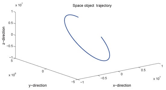
Figure 10.
Space target trajectory.
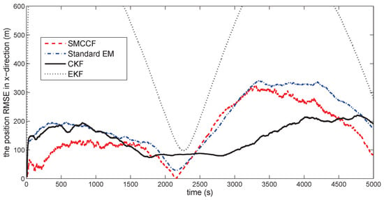
Figure 11.
The position RMSE in the x-direction.
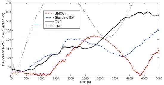
Figure 12.
The position RMSE in the y-direction.
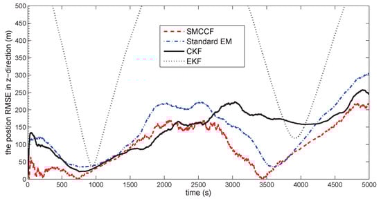
Figure 13.
The position RMSE in the z-direction.
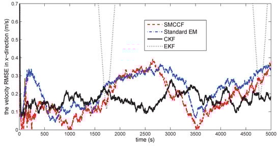
Figure 14.
The velocity RMSE in the x-direction.
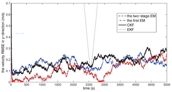
Figure 15.
The velocity RMSE in the y-direction.
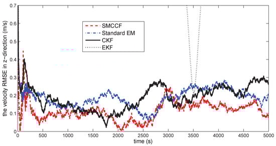
Figure 16.
The velocity RMSE in the z-direction.

Table 1.
RMSE comparison.
7. Conclusions
In the case that a UI is associated with the system state, UI estimation requires the FTM at least. For these dynamic systems with the above-considered UI forms, this paper proposes a novel SMCCF based on a two-stage EM framework, which further improves the state estimation performance by fitting the UI-FTM and using it to simultaneously correct the state estimation and its covariance. Through a space target orbit tracking example, the superiority of SMCCF, as compared to the standard NESs or EM algorithms, is demonstrated.
Author Contributions
Xiaoxu Wang contributes to the idea of the orbit state estimation using the SMCCF and to the algorithm performance demonstration. Quan Pan and Zhengtao Ding contribute to the framework design and the computation programme of the SMCCF, respectively. Zhengya Ma contributes to the software design and the manuscript editing.
Funding
This work was supported in part by the National Natural Science Foundation of China under Grants 61573287, 61203234, 61135001, and 61374023, in part by the Shaanxi Natural Science Foundation of China under Grant 2017JM6006, in part by the Aviation Science Foundation of China under Grant 2016ZC53018, in part by the Fundamental Research Funds for Central Universities under Grants 3102017jghk02009, 3102018AX002 and in part by the Equipment Pre-research Foundation under Grant 2017-HT-XG.
Acknowledgments
The author would like to thank Yonggang Wang for providing the MATLAB programs in the simulation analysis.
Conflicts of Interest
The authors declare no conflict of interest.
References
- Crassidis, J.L.; Junkin, J. Optimal Estimation of Dynamic Systems; Chapman & Hall/CRC: Boca Raton, FL, USA, 2012; Volume 10, p. xiv 591. [Google Scholar]
- Prussing, J.E.; Conway, B.A. Continuous-Thrust Orbit Transfer. In Orbital Mechanics; Oxford University Press: New York, NY, USA, 1993; pp. 283–325. ISBN 978-0-19-983770-0. [Google Scholar]
- Arasaratnam, I.; Haykin, S. Cubature Kalman smoother. Automatica 2011, 47, 2245–2250. [Google Scholar] [CrossRef]
- Ito, K.; Xiong, K. Gaussian filters for nonlinear filtering problems. Autom. Control IEEE Trans. 2000, 45, 910–927. [Google Scholar] [CrossRef]
- Horwood, J.T.; Poore, A.B. Adaptive Gaussian Sum Filters for Space Surveillance. IEEE Trans. Autom. Control 2011, 56, 1777–1790. [Google Scholar] [CrossRef]
- Lan, H.; Liang, Y.; Yang, F.; Wang, Z.; Pan, Q. Joint estimation and identification for stochastic systems with unknown inputs. Control Theory Appl. IET 2013, 7, 1377–1386. [Google Scholar] [CrossRef]
- Wang, Y.G.; Wang, X.; Pan, Q.; Liang, Y. Covariance correction filter with unknown disturbance associated to system state. In Proceedings of the American Control Conference (ACC), Boston, MA, USA, 6–8 July 2016; Volume 10, pp. 3632–3637. [Google Scholar]
- Dempster, A.P.; Laird, N.M.; Rubin, D.B. Maximum Likelihood from Incomplete Data via the EM Algorithm. J. R. Stat. Soc. 1977, 39, 1–38. [Google Scholar]
- Wang, X.X.; Liang, Y.; Pan, Q. Measurement random latency probability identification. IEEE Trans. Autom. Control 2016, 61, 4210–4216. [Google Scholar] [CrossRef]
- Rauch, H.E. Solutions to the linear smoothing problem. IEEE Trans. Autom. Control 1963, 8, 371–372. [Google Scholar] [CrossRef]
- Wan, E.A.; van der R Merwe, L. The Unscented Kalman Filter. In Kalman Filtering and Neural Networks; Simon Haykin, F., Ed.; Wiley: New York, NY, USA, 2001; pp. 221–273. ISBN 0-471-36998-5. [Google Scholar]
- Simo, S. Unscented Rauchung triebel Smoother. IEEE Trans. Autom. Control 2008, 53, 845–849. [Google Scholar]
- Wang, X.X.; Song, B.; Liang, Y.; Pan, Q. EM-based Adaptive Divided Difference Filter for Nonlinear System with Multiplicative Parameter. Int. J. Robust Nonlinear Control 2016, 27, 2167–2197. [Google Scholar] [CrossRef]
- Wang, X.X.; Liang, Y.; Pan, Q.; Zhao, C.H.; Yang, F. Nonlinear Gaussian smoothers with colored measurement noise. IEEE Trans. Autom. Control 2015, 60, 870–876. [Google Scholar] [CrossRef]
- Wang, X.X.; Pan, Q.; Liang, Y.; Yang, F. Gaussian smoothers for nonlinear systems with one-step randomly delayed measurements. IEEE Trans. Autom. Control 2013, 58, 1828–1835. [Google Scholar] [CrossRef]
- Wang, X.X.; Liang, Y.; Pan, Q.; Zhao, C.H.; Yang, F. Design and implementation of Gaussian filter for nonlinear system with randomly delayed measurements and correlated noises. Appl. Math. Comput. 2014, 232, 1011–1024. [Google Scholar] [CrossRef]
- Wang, X.X.; Liang, Y.; Pan, Q.; Yang, F. A Gaussian approximation recursive filter for nonlinear systems with correlated noises. Automatica 2012, 48, 2290–2297. [Google Scholar] [CrossRef]
- Mazya, V.; Schmidt, G. On approximate approximations using gaussian kernels. IMA J. Numer. Anal. 1996, 16, 13–29. [Google Scholar] [CrossRef]
- Douza, A.A. Using EM to estimate a probablity density with a mixture of gaussians. Available online: https://www-clmc.usc.edu/~adsouza/notes/mix_gauss.pdf (accessed on 17 May 1999).
© 2018 by the authors. Licensee MDPI, Basel, Switzerland. This article is an open access article distributed under the terms and conditions of the Creative Commons Attribution (CC BY) license (http://creativecommons.org/licenses/by/4.0/).