Comparing Building and Neighborhood-Scale Variability of CO2 and O3 to Inform Deployment Considerations for Low-Cost Sensor System Use


Abstract
1. Introduction and Background
2. Materials & Methods
2.1. Deployment Overview (Sensor Systems, Siting, and Timeline)
2.2. Signal Processing and Sensor Quantification
2.2.1. Quantification of CO2 Sensors
2.2.2. Quantification of the O3 Sensors
3. Results and Discussion
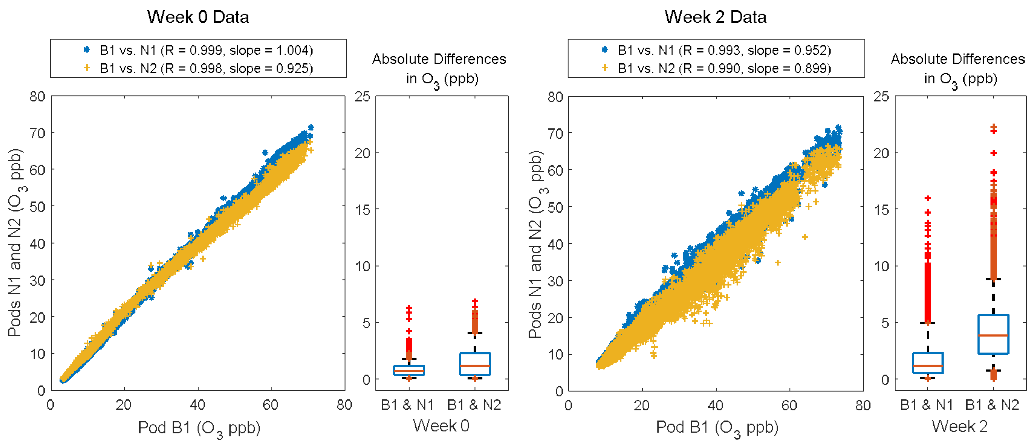
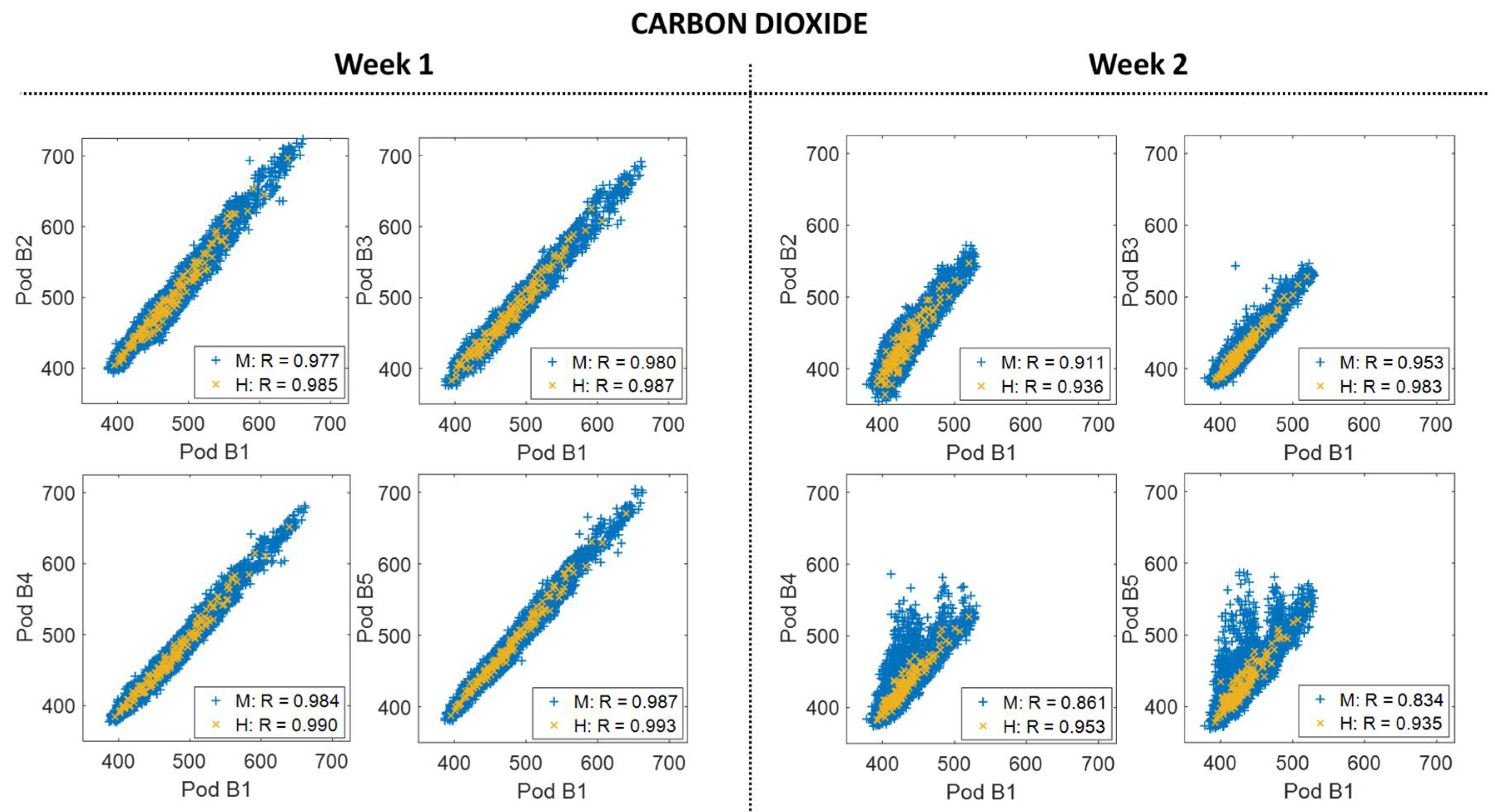
3.1. Field Calibration Results (Sensor System Uncertainty)
3.2. Neighborhood-Scale Variability
3.3. Building-Scale Variability
3.4. Impact of Siting Choices on Neighborhood Varibaility Analysis
3.5. Generalizability of Building-Scale Spatial Variability & Potential Recommendations
- Compare Sensors: Co-locating sensors in the field will support a better understanding of inter-sensor variability prior to their deployment, which will aid in attributing new variability introduced by the deployment of sensor systems to separate sites. These relative comparisons can also be valuable if there are problems with the calibration.
- Placement and Distribution: To study a particular emission source, place sensors upwind and downwind of the site of interest, at varying distances. Some of the sensors should have a line of sight to the emission source. Consider factors such as typical wind directions and potential obstructions, which may impact the transport of emissions. These placements should also minimize added variability when possible. For example, shading all sensor systems, placing them on the same sides of buildings, or placing them exclusively on rooftops could reduce the variability and biases that result from occasional direct sunlight.
- Supplementary Materials Sensor Data: Consider using multiple systems or sensor types. The ability of sensors to capture variability on small spatial scales could be leveraged to aid in source identification by placing multiple sensor systems at a site with the objective of capturing local emissions with some systems and targeting exclusively regional trends with other systems. Leveraging data from multiple sensor types could also shed light on sources and emissions by studying the correlations or temporal patterns of data from sensors intended to measure different target pollutants.
- Document Deployment: Document your deployment in writing and with photos (take photos of the sensor systems from different angles and photos from the sensors of what they “see”). Learning about nearby activities could provide contextual information that can aid in data interpretation and reduce the misinterpretation of sensor data.
4. Conclusions
Supplementary Materials
Author Contributions
Acknowledgments
Conflicts of Interest
Appendix A. Sensor Quantification Results

| Carbon Dioxide | Ozone | |||||||||||
|---|---|---|---|---|---|---|---|---|---|---|---|---|
| Training Data | Testing Data | Training Data | Testing Data | |||||||||
| Pod | R2 | RMSE | MB | R2 | RMSE | MB | R2 | RMSE | MB | R2 | RMSE | MB |
| B2 | 0.93 | 7.32 | −0.01 | 0.94 | 9.69 | −6.35 | NA | NA | NA | NA | NA | NA |
| B3 | 0.93 | 7.85 | −0.04 | 0.93 | 7.39 | 2.69 | 0.97 | 3.45 | −0.11 | 0.94 | 5.16 | −1.88 |
| B4 | 0.86 | 11.2 | 0.01 | 0.83 | 11.3 | 5.84 | 0.96 | 3.88 | −0.07 | 0.96 | 4.73 | −2.18 |
| B5 | 0.94 | 7.35 | −0.03 | 0.92 | 7.25 | 1.90 | 0.96 | 4.00 | −0.11 | 0.92 | 6.51 | −3.07 |
| B7 | 0.94 | 7.32 | 0.01 | 0.77 | 14.7 | 10.4 | 0.97 | 3.71 | −0.13 | 0.94 | 5.30 | −1.99 |
| B8 | 0.91 | 9.11 | −0.04 | 0.88 | 9.00 | 0.39 | 0.98 | 2.78 | −0.08 | 0.97 | 3.96 | −0.94 |
| C9 | 0.88 | 10.3 | −0.04 | 0.89 | 14.6 | 12.8 | 0.97 | 3.74 | −0.08 | 0.95 | 5.10 | −2.96 |
| D2 | 0.95 | 6.19 | −0.02 | 0.93 | 6.83 | 3.49 | 0.96 | 3.95 | −0.08 | 0.93 | 6.21 | −3.08 |
| Ave | 0.92 | 8.33 | −0.02 | 0.89 | 10.1 | 3.89 | 0.97 | 3.65 | −0.09 | 0.94 | 5.28 | −2.30 |
| SD | 0.03 | 1.71 | 0.02 | 0.06 | 3.16 | 5.95 | 0.01 | 0.42 | 0.02 | 0.02 | 0.86 | 0.79 |

Appendix B. Additional Figures and Time Series of Data Used for Analysis


References
- Jerrett, M.; Donaire-Gonzalez, D.; Popoola, O.; Jones, R.; Cohen, R.C.; Almanza, E.; de Nazelle, A.; Mead, I.; Caarrasco-Turigas, G.; Cole-Hunter, T.; et al. Validating novel air pollution sensors to improve exposure estimates for epidemiological analyses and citizen science. Environ. Res. 2017, 158, 286–294. [Google Scholar] [CrossRef] [PubMed]
- Sadighi, K.; Coffey, E.; Polidori, A.; Feenstra, B.; Lv, Q.; Henze, D.K.; Hannigan, M. Intra-urban spatial variability of surface ozone and carbon dioxide in Riverside, CA: Viability and validation of low-cost sensors. Atmos. Meas. Tech. Discuss. 2017. [Google Scholar] [CrossRef]
- Mead, M.I.; Popoola, O.A.M.; Stewart, G.B.; Landshoff, P.; Calleja, M.; Hayes, M.; Baldovi, J.J.; McLeod, M.W.; Hodgson, T.F.; Dicks, J.; et al. The use of electrochemical sensors for monitoring urban air quality in low-cost, high-density networks. Atmos. Environ. 2013, 70, 186–203. [Google Scholar] [CrossRef]
- Piedrahita, R.; Xiang, Y.; Masson, N.; Ortega, J.; Collier, A.; Jiang, Y.; Li, K.; Dick, R.P.; Lv, Q.; Hannigan, M.; et al. The next generation of low-cost personal air quality sensors for quantitative exposure monitoring. Atmos. Meas. Tech. 2014, 7, 3325–3336. [Google Scholar] [CrossRef]
- Zimmerman, N.; Presto, A.A.; Kumar, S.P.N.; Gu, J.; Hauryliuk, A.; Robinson, E.S.; Robinson, A.L.; Subramanian, R. A machine learning calibration model using random forests to improve sensor performance for lower-cost air quality monitoring. Atmos. Meas. Tech. 2018, 11, 291–313. [Google Scholar] [CrossRef]
- Cross, E.S.; Williams, L.R.; Lewis, D.K.; Magoon, G.R.; Onasch, T.B.; Kaminsky, M.L.; Worsnop, D.R.; Jayne, J.T. Use of electrochemical sensors for measurement of air pollution: Correcting interference response and validating measurements. Atmos. Meas. Tech. 2017, 10, 3575–3588. [Google Scholar] [CrossRef]
- Kim, J.; Shusterman, A.A.; Lieschke, K.J.; Newman, C.; Cohen, R.C. The berkeley atmospheric CO2 observation network: Field calibration and evaluation of low-cost air quality sensors. Atmos. Meas. Tech. Discuss. 2017. [Google Scholar] [CrossRef]
- Vardoulakis, S.; Gonzalez-Flesca, N.; Fisher, B.E.A.; Pericleous, K. Spatial variability of air pollution in the vicinity of a permanent monitoring station in central Paris. Atmos. Environ. 2005, 39, 2725–2736. [Google Scholar] [CrossRef]
- Croxford, B.; Penn, A. Siting considerations for urban pollution monitors. Atmos. Environ. 1998, 32, 1049–1057. [Google Scholar] [CrossRef]
- Miskell, G.; Salmond, J.; Williams, D.E. Science of the total environment low-cost sensors and crowd-sourced data: Observations of siting impacts on a network of air-quality instruments. Sci. Total Environ. 2017, 575, 1119–1129. [Google Scholar] [CrossRef] [PubMed]
- Williams, R.; Kilaru, V.; Snyder, E.; Kaufman, A.; Dye, T.; Rutter, A.; Russell, A.; Hafner, H. Air Sensor Guidebook; EPA/600/R-14/159 (NTIS PB2015-100610); U.S. Environmental Protection Agency: Washington, DC, USA, 2014.
- AQ-SPEC Air Quality Sensor Performance Evaluation Center (SCAQMD). Available online: http://www.aqmd.gov/aq-spec/home (accessed on 9 March 2018).
- Air Sensor Workgroup (EDF). Available online: https://www.edf.org/health/air-sensor-workgroup (accessed on 9 March 2018).
- Clements, A.L.; Griswold, W.G.; RS, A.; Johnston, J.E.; Herting, M.M.; Thorson, J.; Collier-Oxandale, A.; Hannigan, M. Low-cost air quality monitoring tools: From research to practice (a workshop summary). Sensors 2017, 17, 2478. [Google Scholar] [CrossRef] [PubMed]
- Casey, J.G.; Collier-Oxandale, A.M.; Hannigan, M.P. Performance of artificial neural networks and linear models to quantify 4 trace gas species in an oil and gas production region with low-cost sensors. Sens. Actuators B 2018, submitted. [Google Scholar]
- Cheadle, L.; Deanes, L.; Sadighi, K.; Casey, J.G.; Collier-Oxandale, A.; Hannigan, M. Quantifying neighborhood-scale spatial variations of ozone at open space and urban sites in Boulder, Colorado using low-cost sensor technology. Sensors 2017, 17, 2072. [Google Scholar] [CrossRef] [PubMed]
- Masson, N.; Piedrahita, R.; Hannigan, M. Quantification method for electrolytic sensors in long-term monitoring of ambient air quality. Sensors 2015, 15, 27283–27302. [Google Scholar] [CrossRef] [PubMed]
- Collier-Oxandale, A.; Hannigan, M.P.; Casey, J.G.; Piedrahita, R.; Ortega, J.; Halliday, H.; Johnston, J. Assessing a low-cost methane sensor quantification system for use in complex rural and urban environments. Atmos. Meas. Tech. Discuss. 2018. [Google Scholar] [CrossRef]
- Masson, N.; Piedrahita, R.; Hannigan, M. Approach for quantification of metal oxide type semiconductor gas sensors used for ambient air quality monitoring. Sens. Actuators B 2015, 208, 339–345. [Google Scholar] [CrossRef]
- Spinelle, L.; Gerboles, M.; Villani, M.G.; Aleixandre, M.; Bonavitacola, F. Field calibration of a cluster of low-cost available sensors for air quality monitoring. Part A: Ozone and nitrogen dioxide. Sens. Actuators B 2015, 215, 249–257. [Google Scholar] [CrossRef]
- Spinelle, L.; Gerboles, M.; Villani, M.G.; Aleixandre, M.; Bonavitacola, F. Field calibration of a cluster of low-cost commercially available sensors for air quality monitoring. Part B: No, CO and CO2. Sens. Actuators B 2017, 238, 706–715. [Google Scholar] [CrossRef]
- Global Greenhouse Gas Reference Network, Trends in Atmospheric Carbon Dioxide (Global Monitoring Division). Available online: https://www.esrl.noaa.gov/gmd/ccgg/trends/ (accessed on 9 March 2018).
- Bart, M.; Williams, D.E.; Ainslie, B.; Mckendry, I.; Salmond, J.; Grange, S.K.; Alavi-Shoshtari, M.; Steyn, D.; Henshaw, G.S. High density ozone monitoring using gas sensitive semi-conductor sensors in the lower Fraser Valley, British Columbia. Environ. Sci. Technol. 2014, 48, 3970–3977. [Google Scholar] [CrossRef] [PubMed]


| Statistic | Training | Testing | |
|---|---|---|---|
| CO2 | R2 | 0.92 (0.03) | 0.89 (0.06) |
| RMSE (ppm) | 8.33 (1.71) | 10.09 (3.16) | |
| MB (ppm) | −0.02 (0.02) | 3.89 (5.95) | |
| O3 | R2 | 0.97 (0.01) | 0.94 (0.02) |
| RMSE (ppb) | 3.65 (0.42) | 5.28 (0.86) | |
| MB (ppb) | −0.09 (0.02) | −2.30 (0.79) |
© 2018 by the authors. Licensee MDPI, Basel, Switzerland. This article is an open access article distributed under the terms and conditions of the Creative Commons Attribution (CC BY) license (http://creativecommons.org/licenses/by/4.0/).
Share and Cite
Collier-Oxandale, A.; Coffey, E.; Thorson, J.; Johnston, J.; Hannigan, M. Comparing Building and Neighborhood-Scale Variability of CO2 and O3 to Inform Deployment Considerations for Low-Cost Sensor System Use. Sensors 2018, 18, 1349. https://doi.org/10.3390/s18051349
Collier-Oxandale A, Coffey E, Thorson J, Johnston J, Hannigan M. Comparing Building and Neighborhood-Scale Variability of CO2 and O3 to Inform Deployment Considerations for Low-Cost Sensor System Use. Sensors. 2018; 18(5):1349. https://doi.org/10.3390/s18051349
Chicago/Turabian StyleCollier-Oxandale, Ashley, Evan Coffey, Jacob Thorson, Jill Johnston, and Michael Hannigan. 2018. "Comparing Building and Neighborhood-Scale Variability of CO2 and O3 to Inform Deployment Considerations for Low-Cost Sensor System Use" Sensors 18, no. 5: 1349. https://doi.org/10.3390/s18051349
APA StyleCollier-Oxandale, A., Coffey, E., Thorson, J., Johnston, J., & Hannigan, M. (2018). Comparing Building and Neighborhood-Scale Variability of CO2 and O3 to Inform Deployment Considerations for Low-Cost Sensor System Use. Sensors, 18(5), 1349. https://doi.org/10.3390/s18051349