Sensor Fusion to Estimate the Depth and Width of the Weld Bead in Real Time in GMAW Processes

 ,
,
Abstract
1. Introduction
2. Materials and Methods
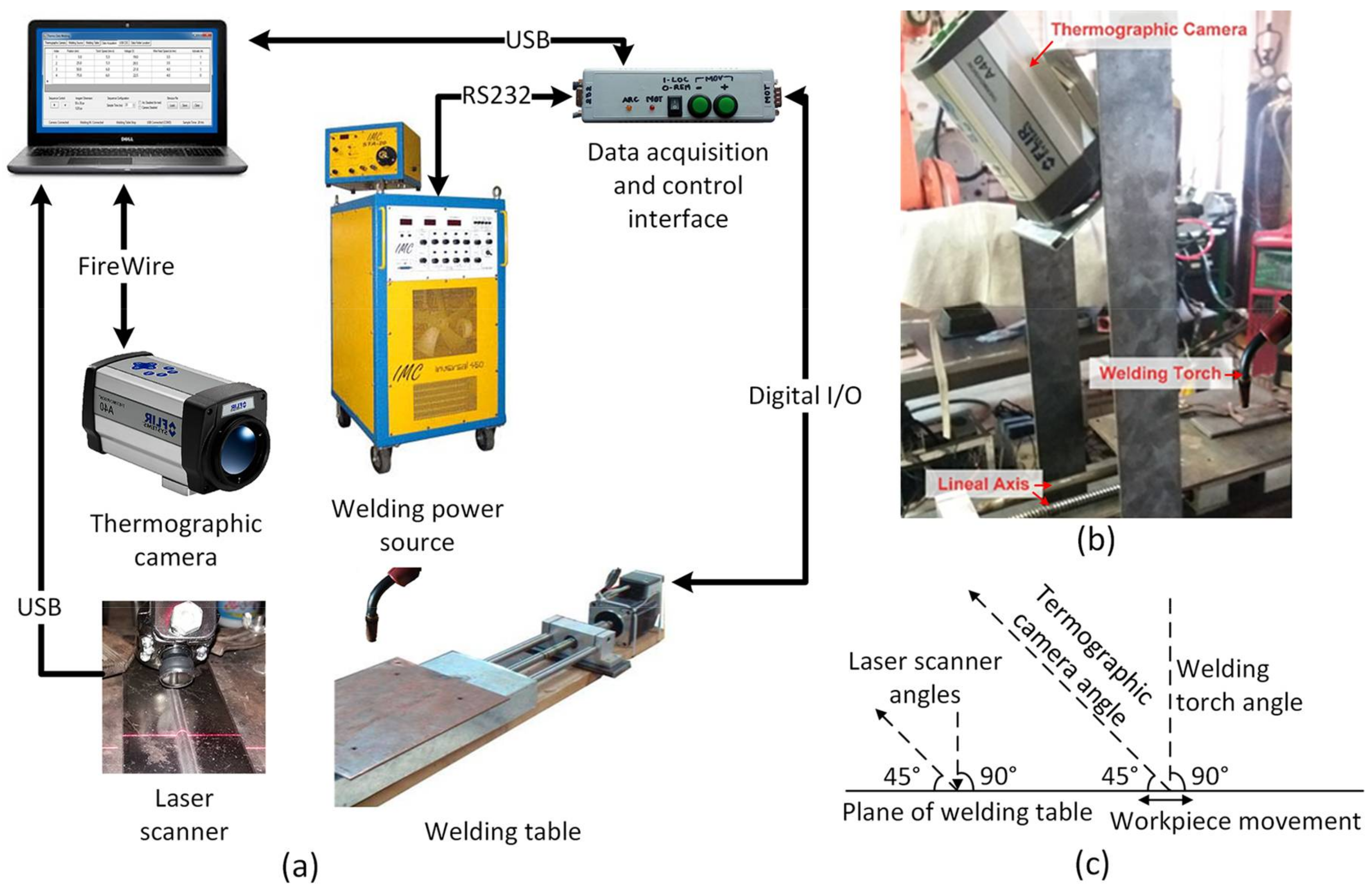
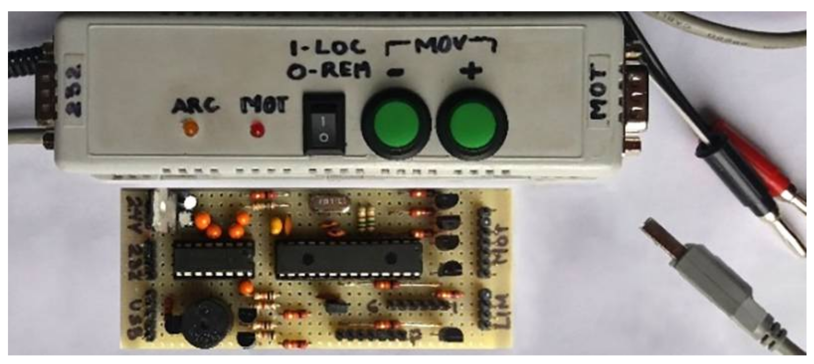
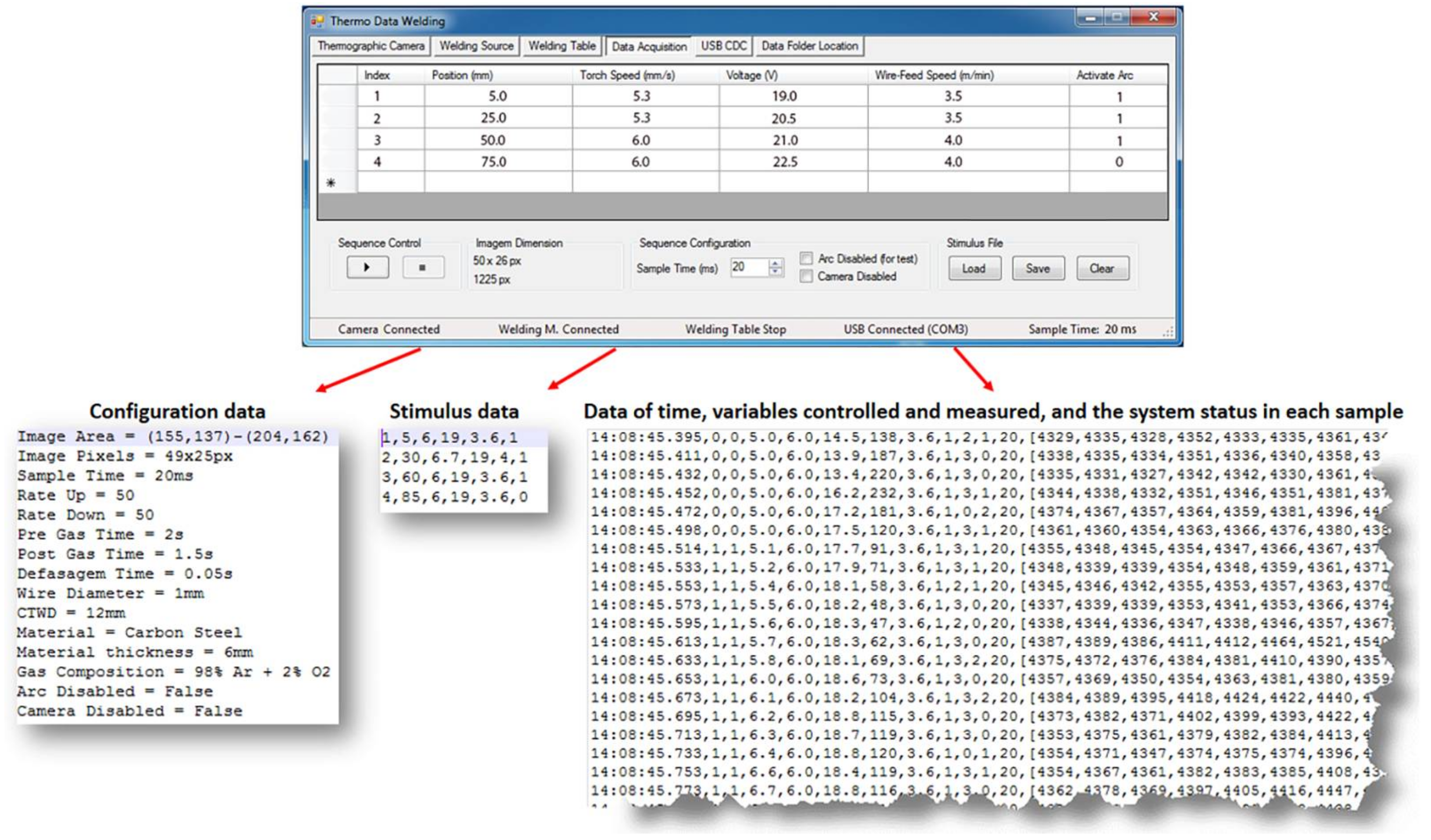
2.1. Data Acquisition and Open-Loop Control System for GMAW Welding Process
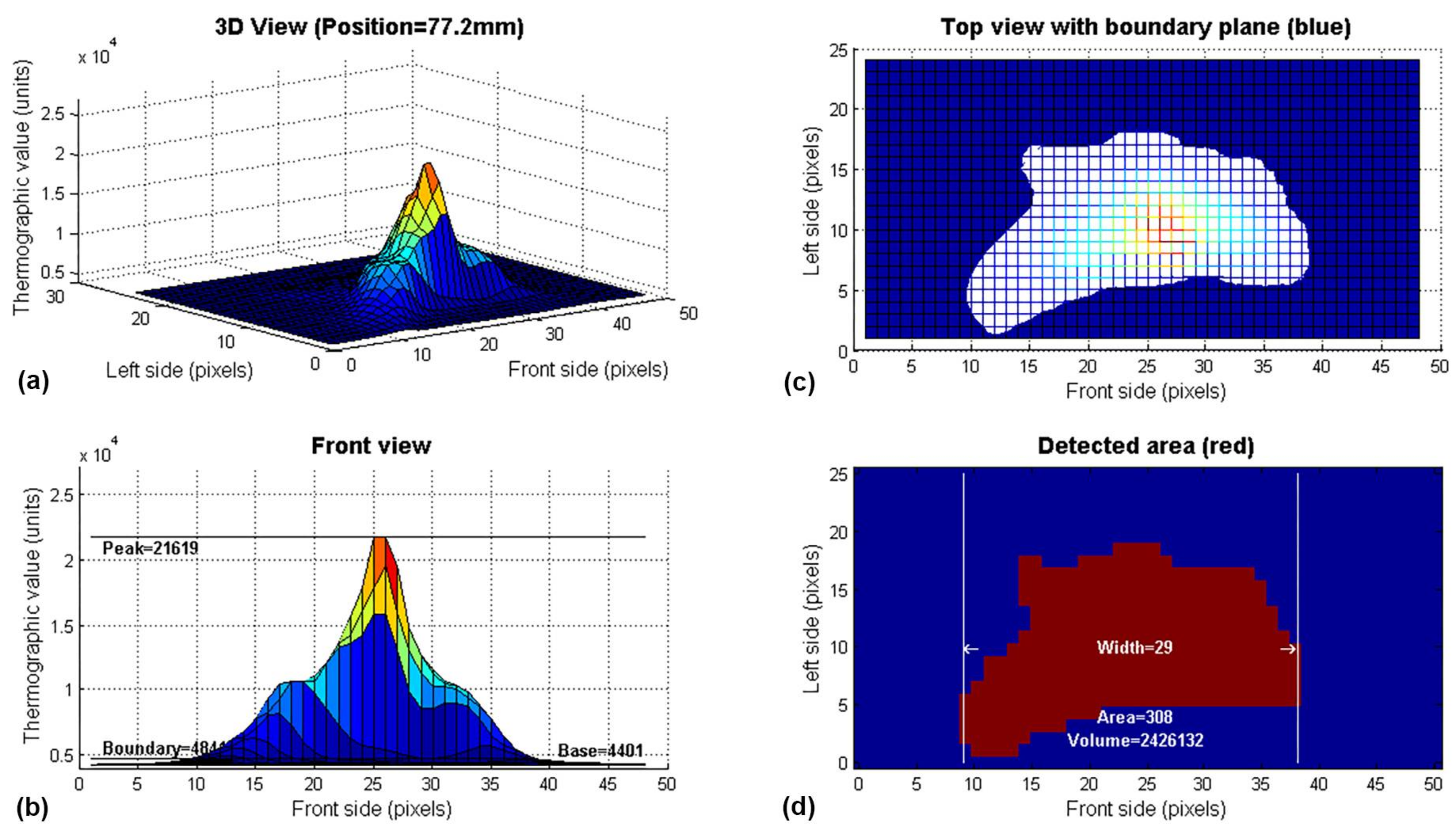
2.2. Infrared Image Features Extraction
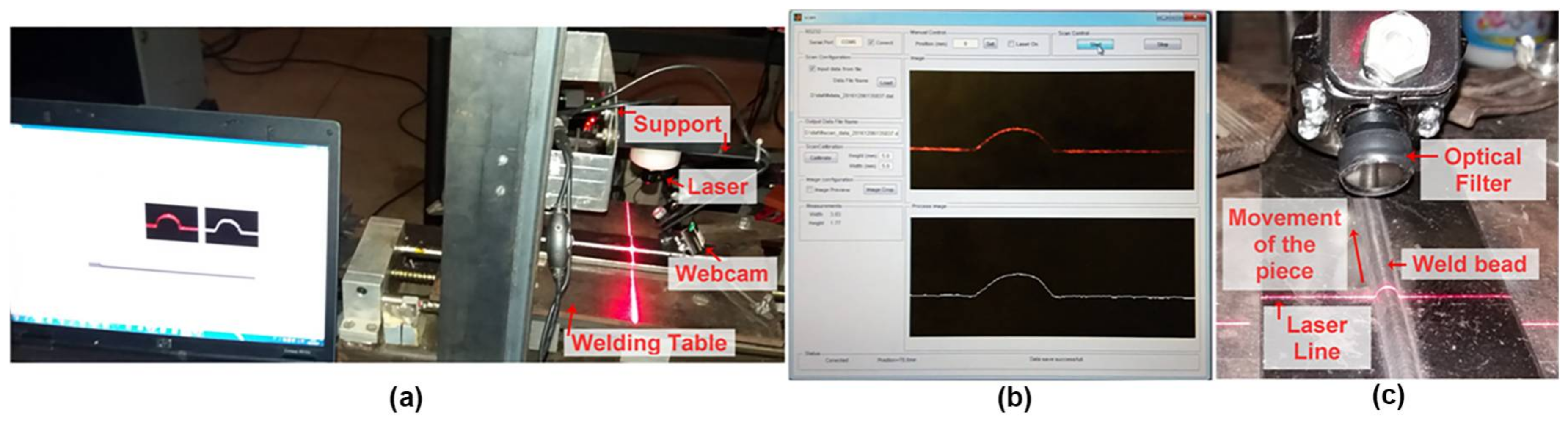
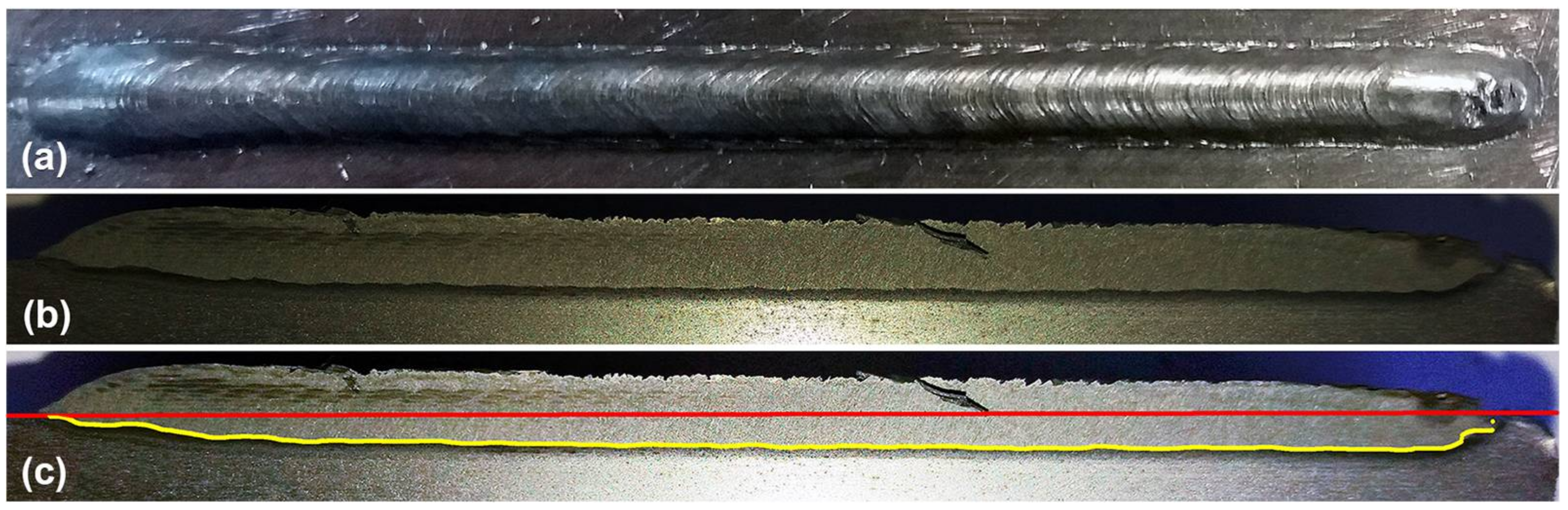
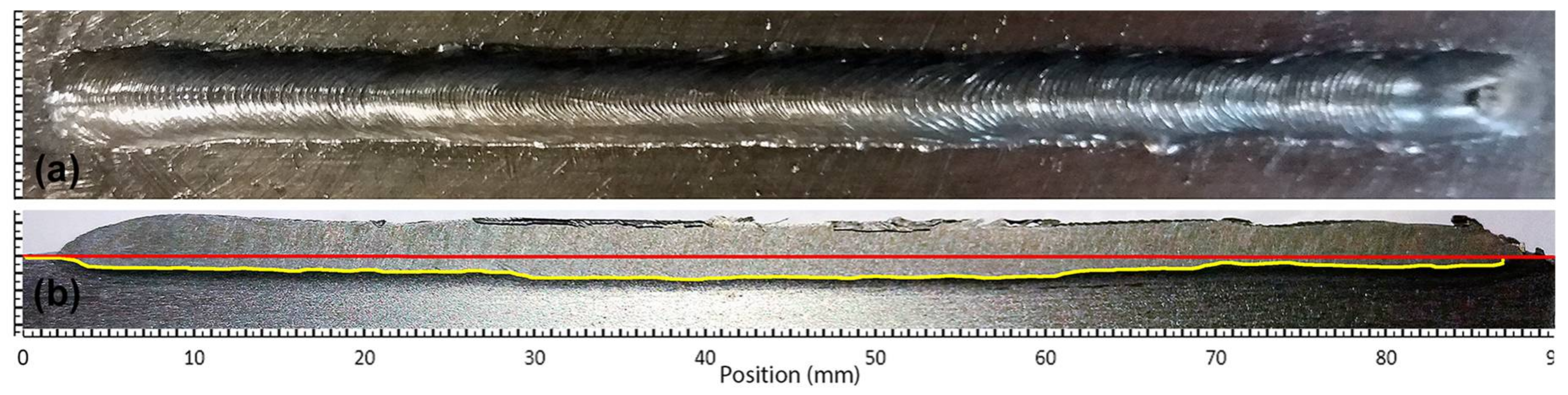
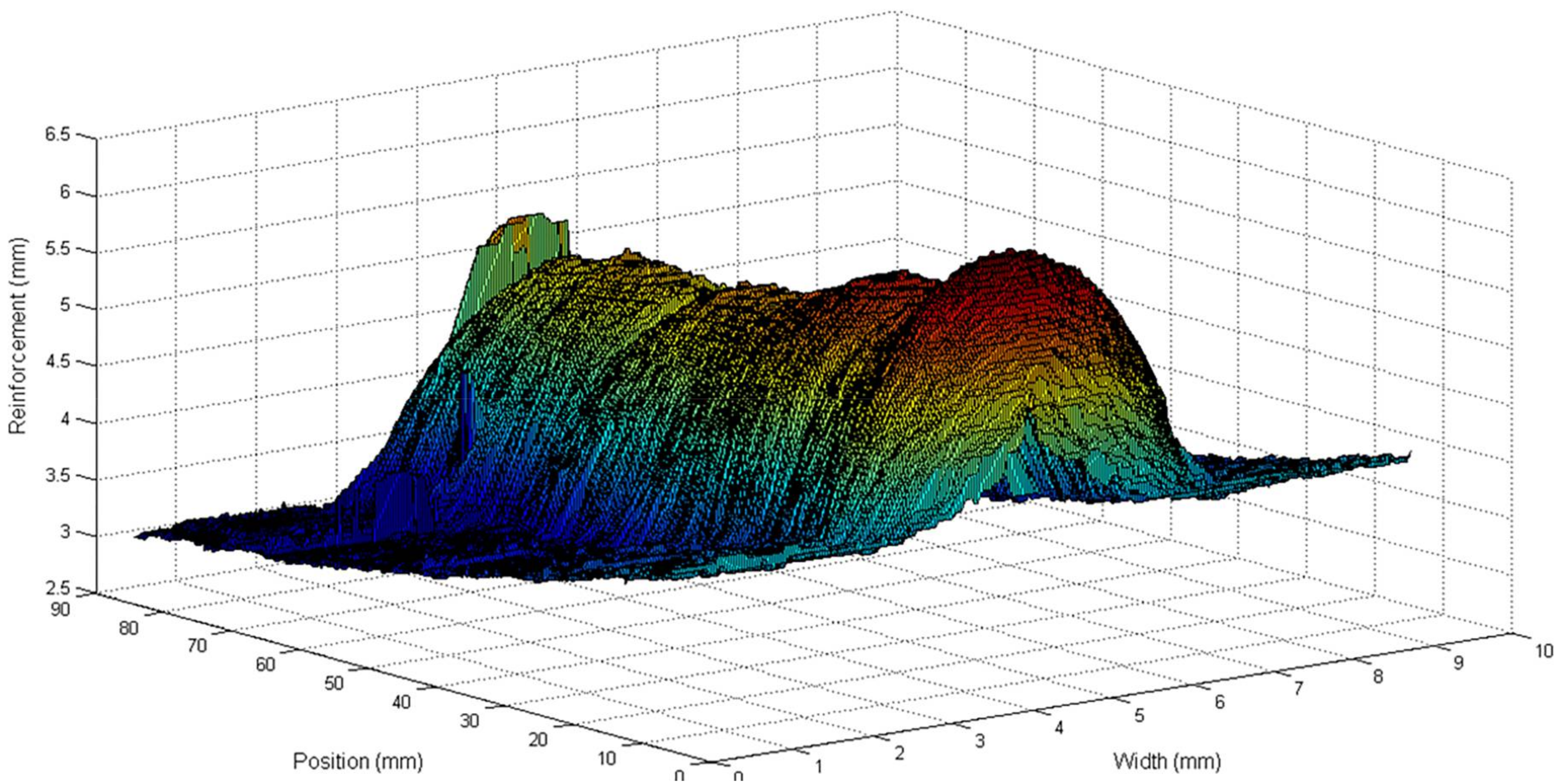
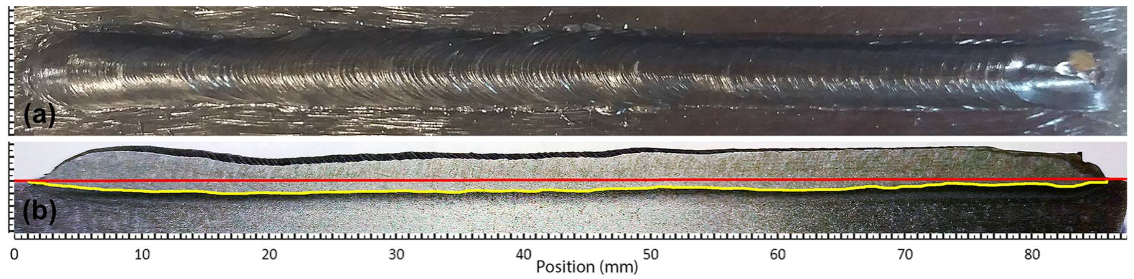
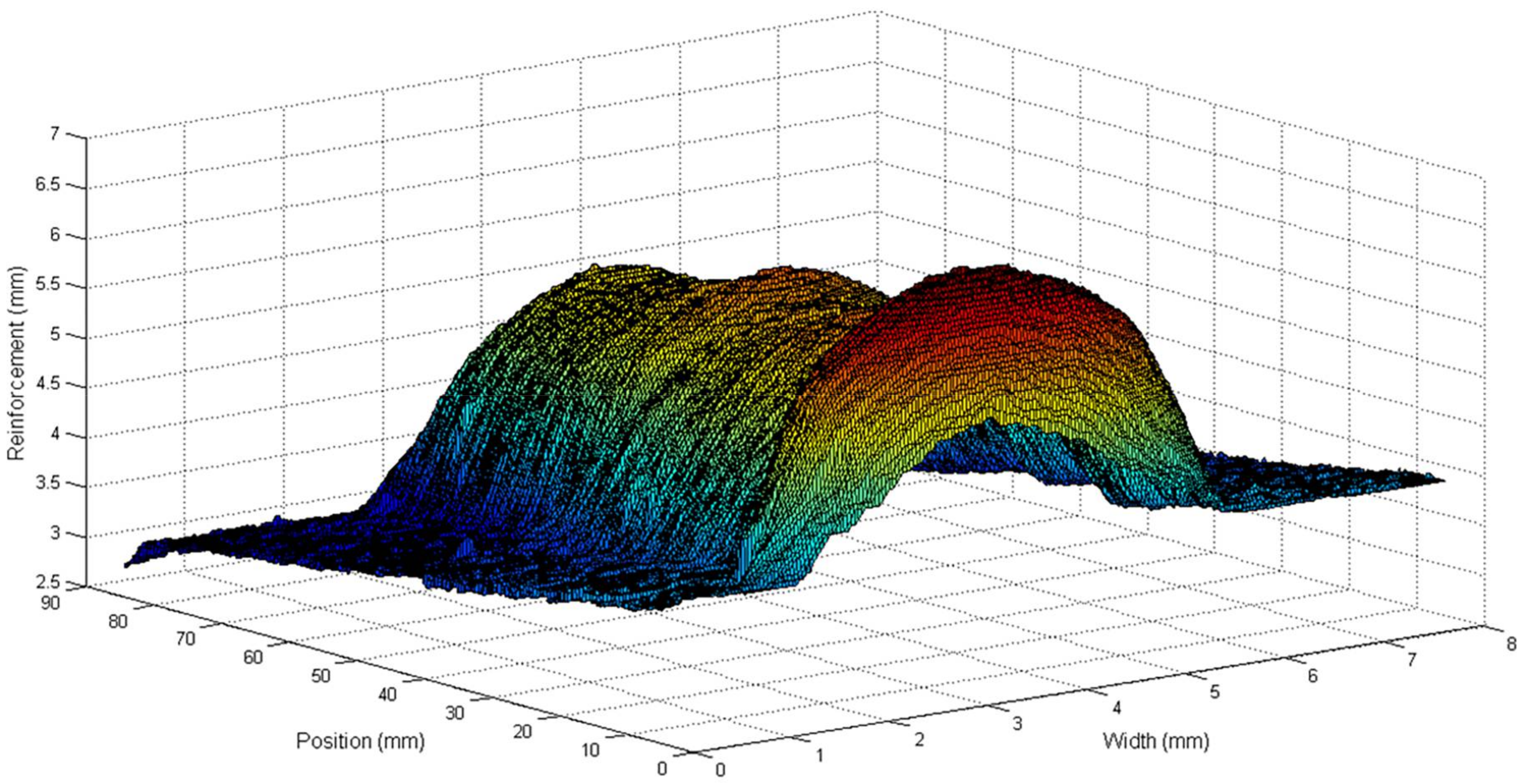
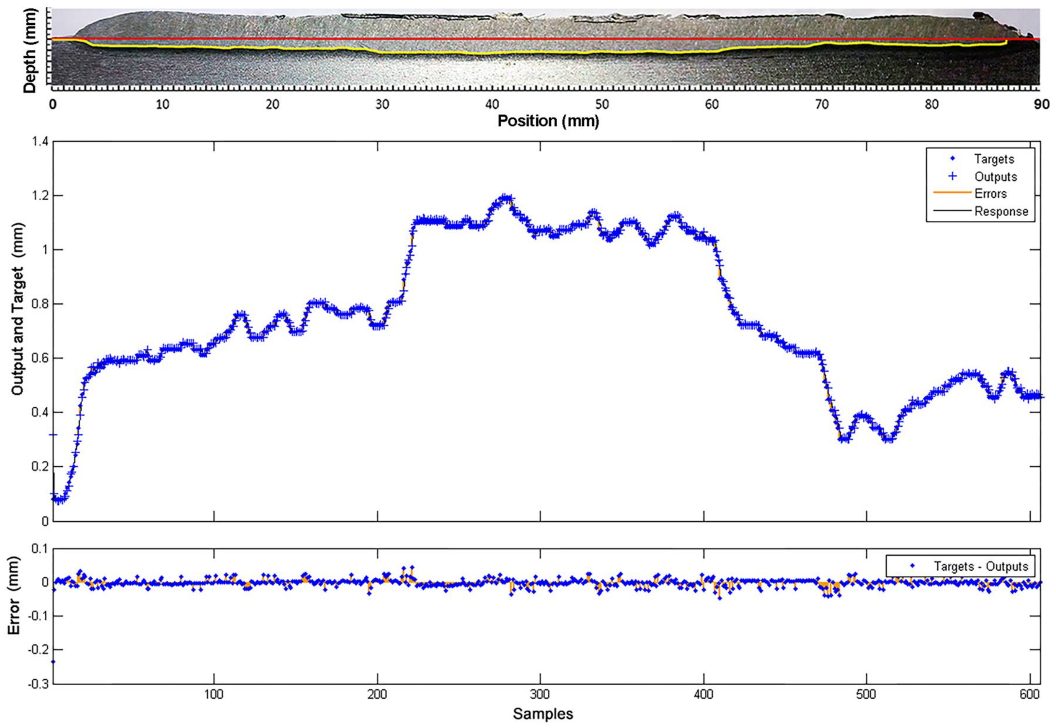
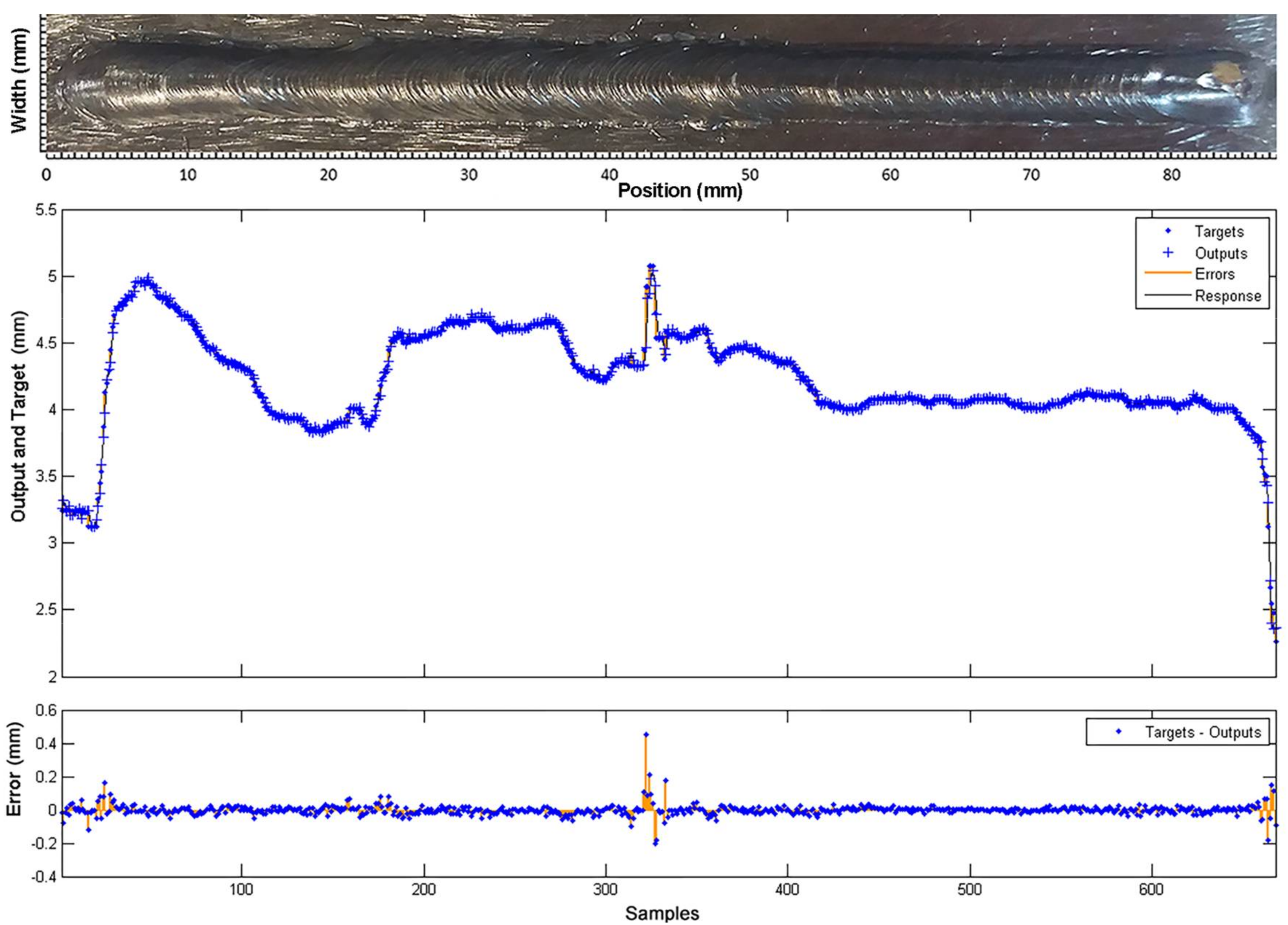
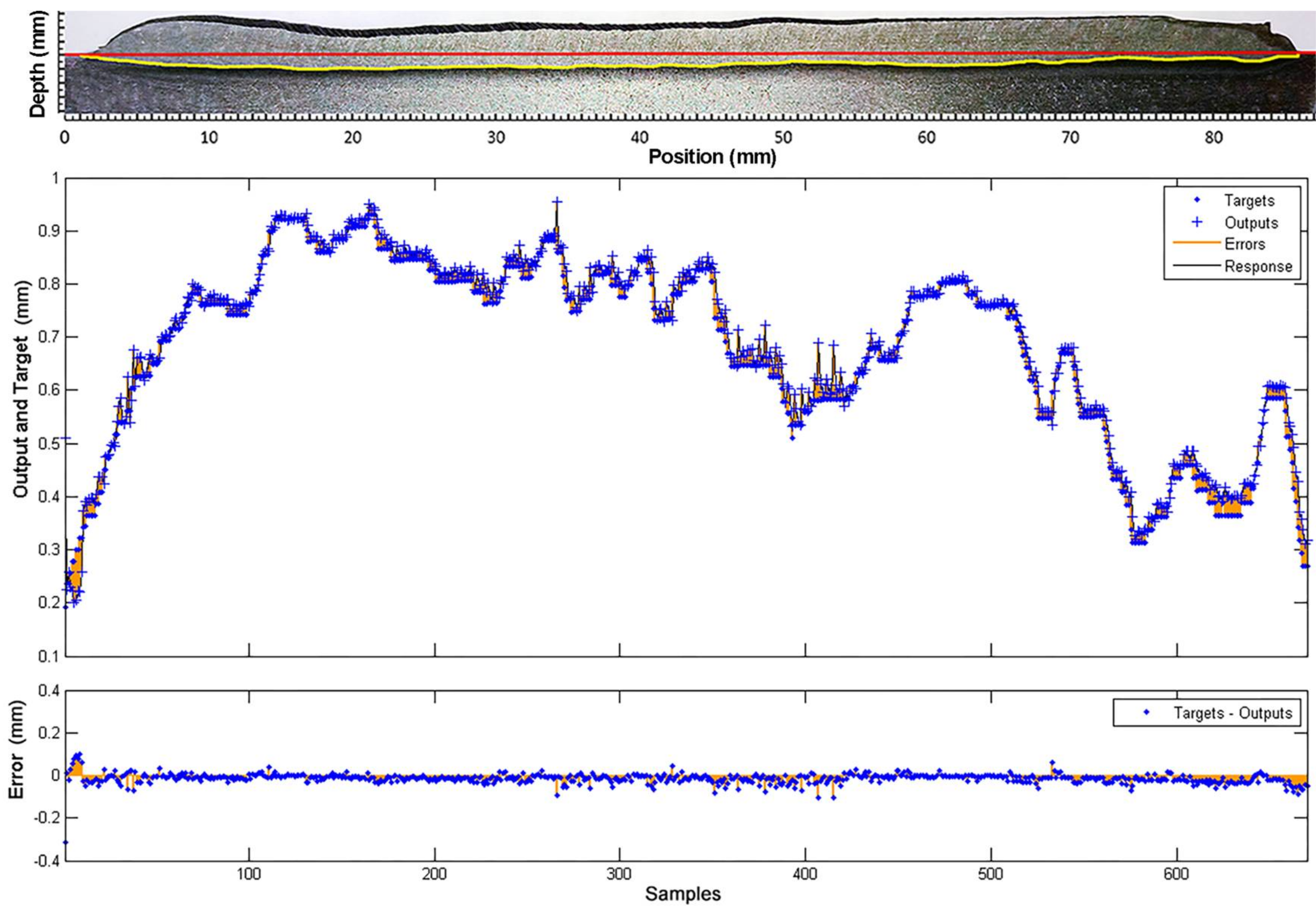
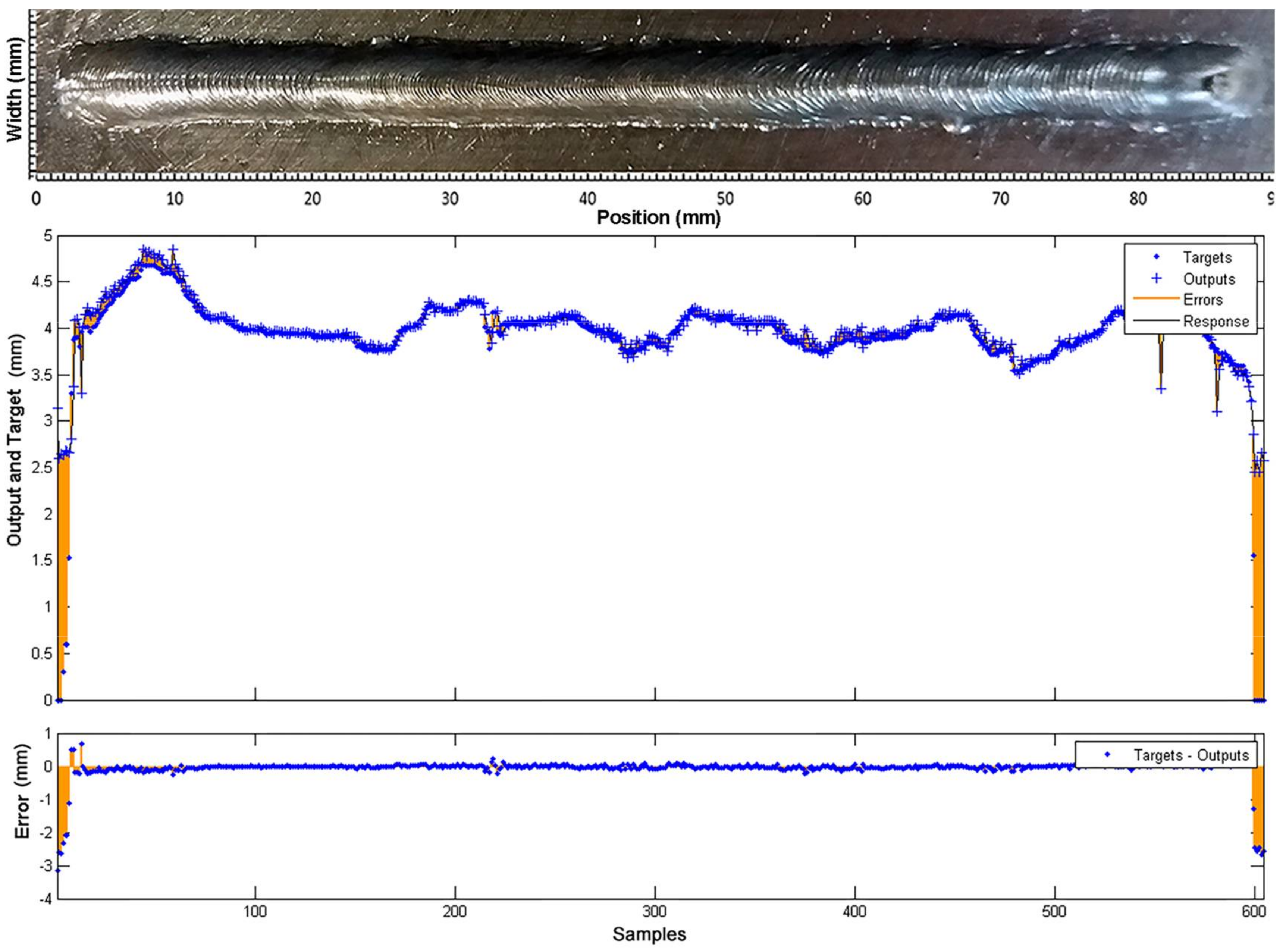
2.3. Laser Scanner and Macrographic Analysis to Obtain the Geometric Profile of the Weld Bead
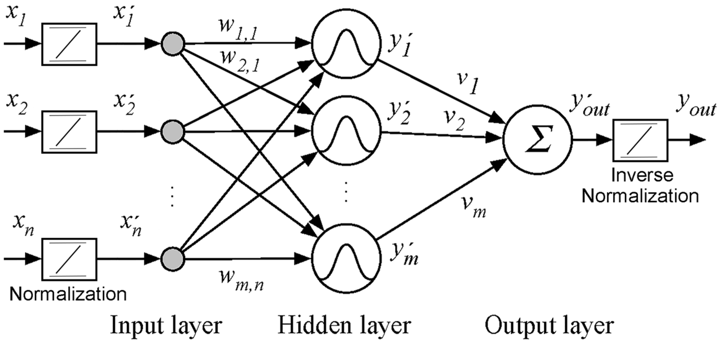
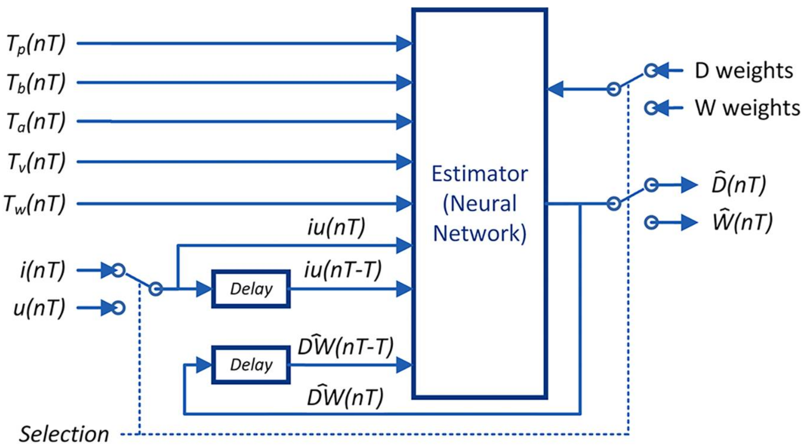
2.4. Sensor Fusion to Estimate the Depth and Width of the Weld Bead
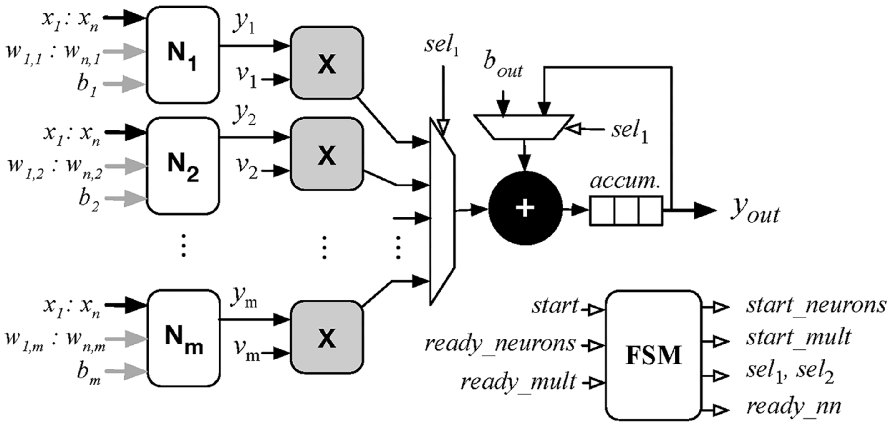
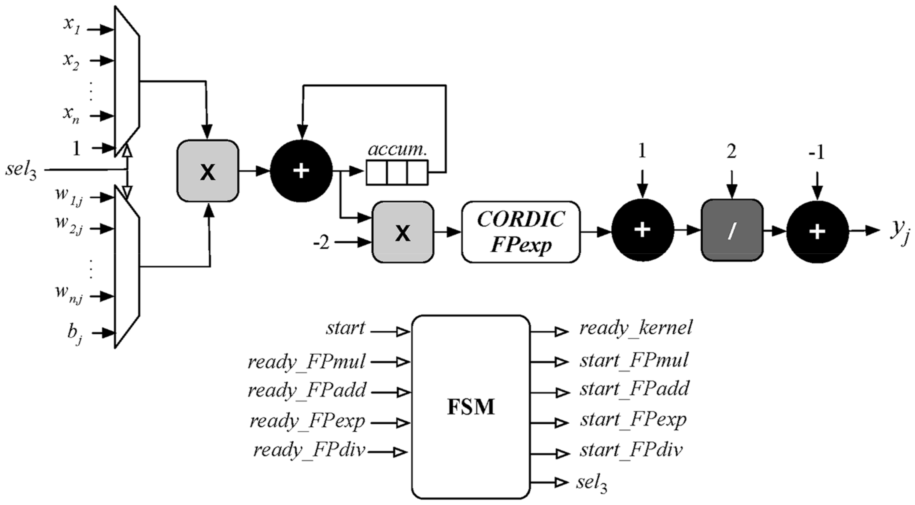
2.5. FPGA Implementation of Weld Bead Depth and Width Estimators
3. Results and Discussion
3.1. Experimental Details
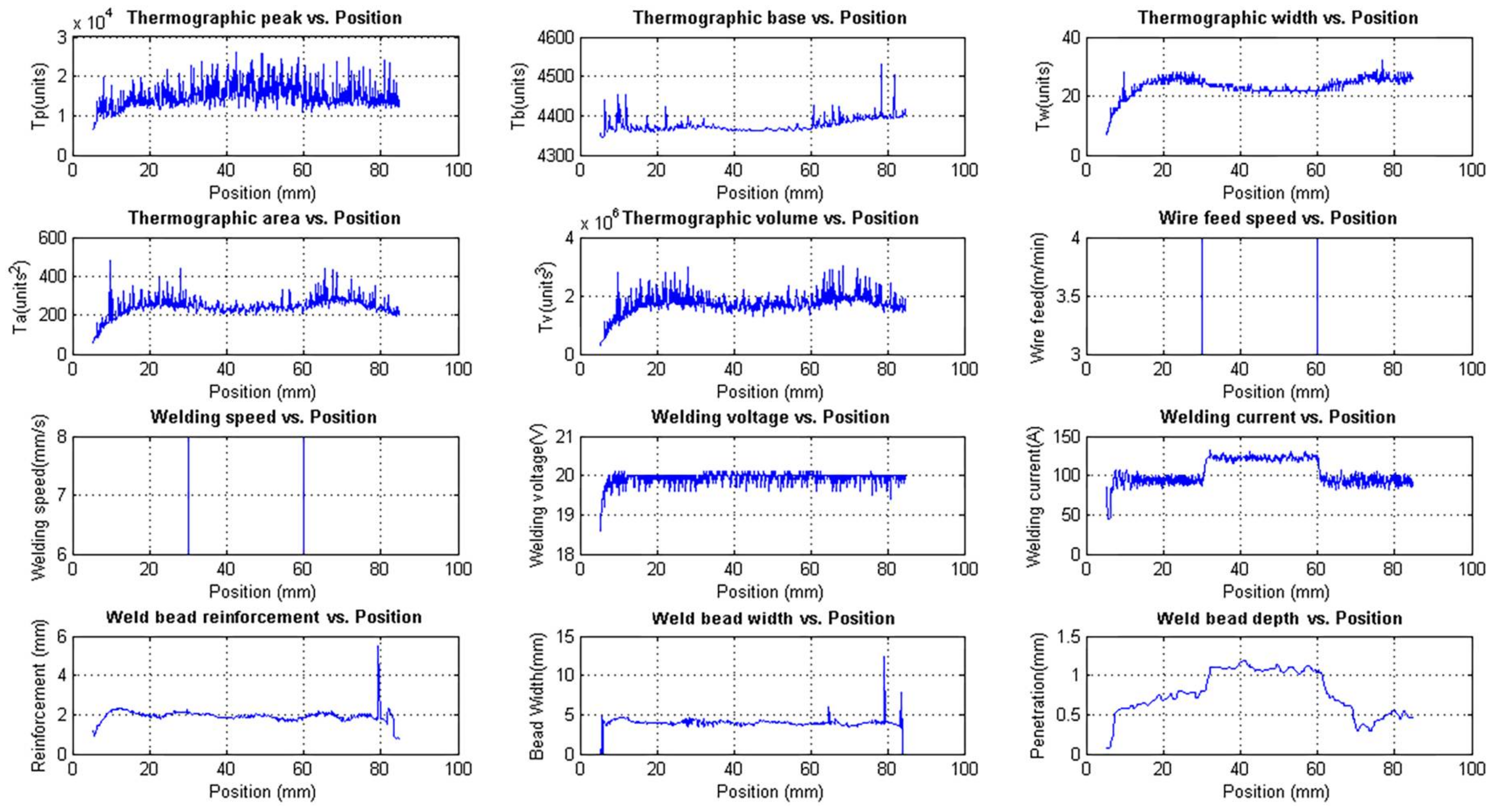
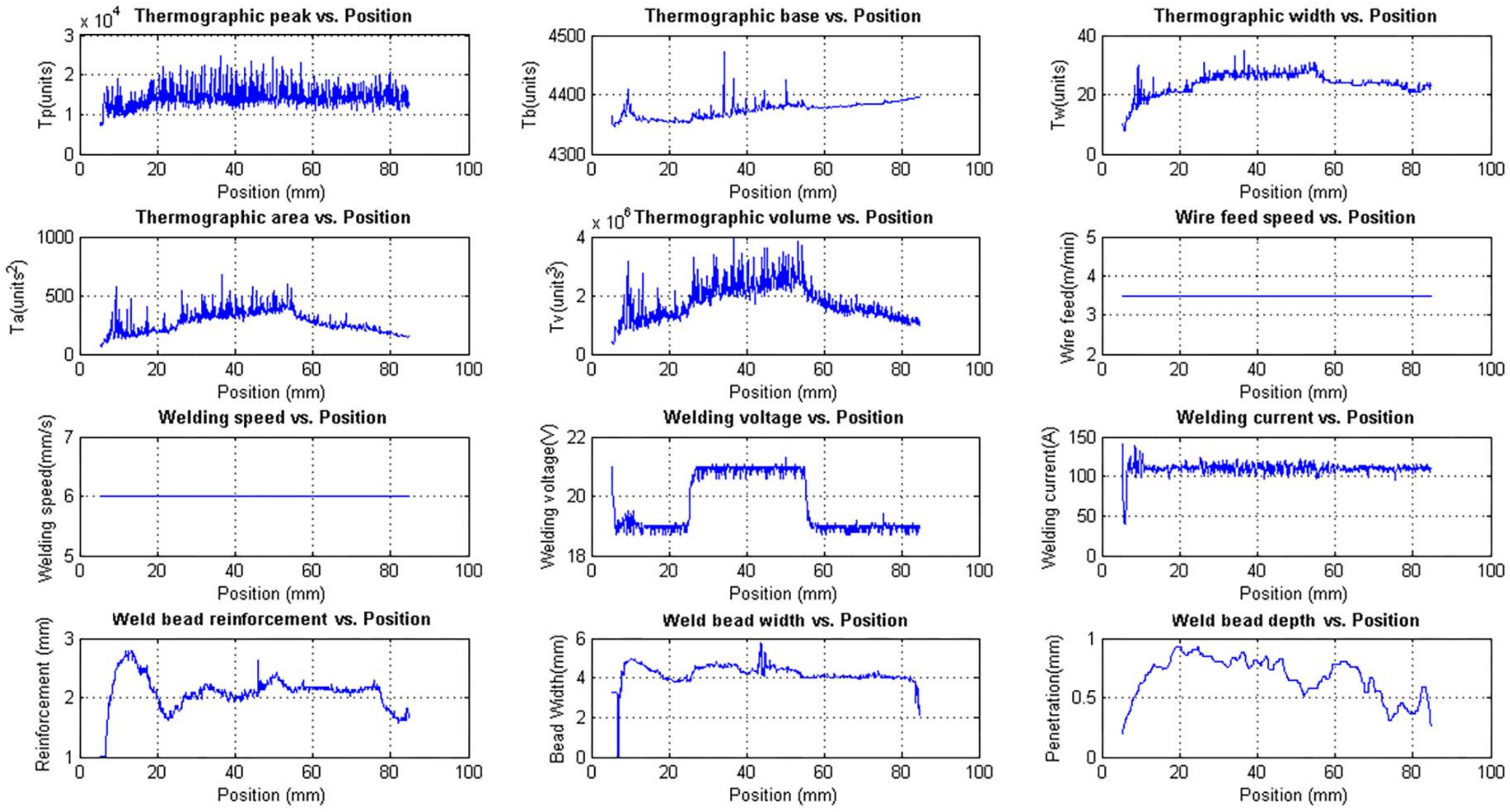
3.1.1. Experiment 1: Process Response to the Step in the Welding Speed and Wire Feed Speed
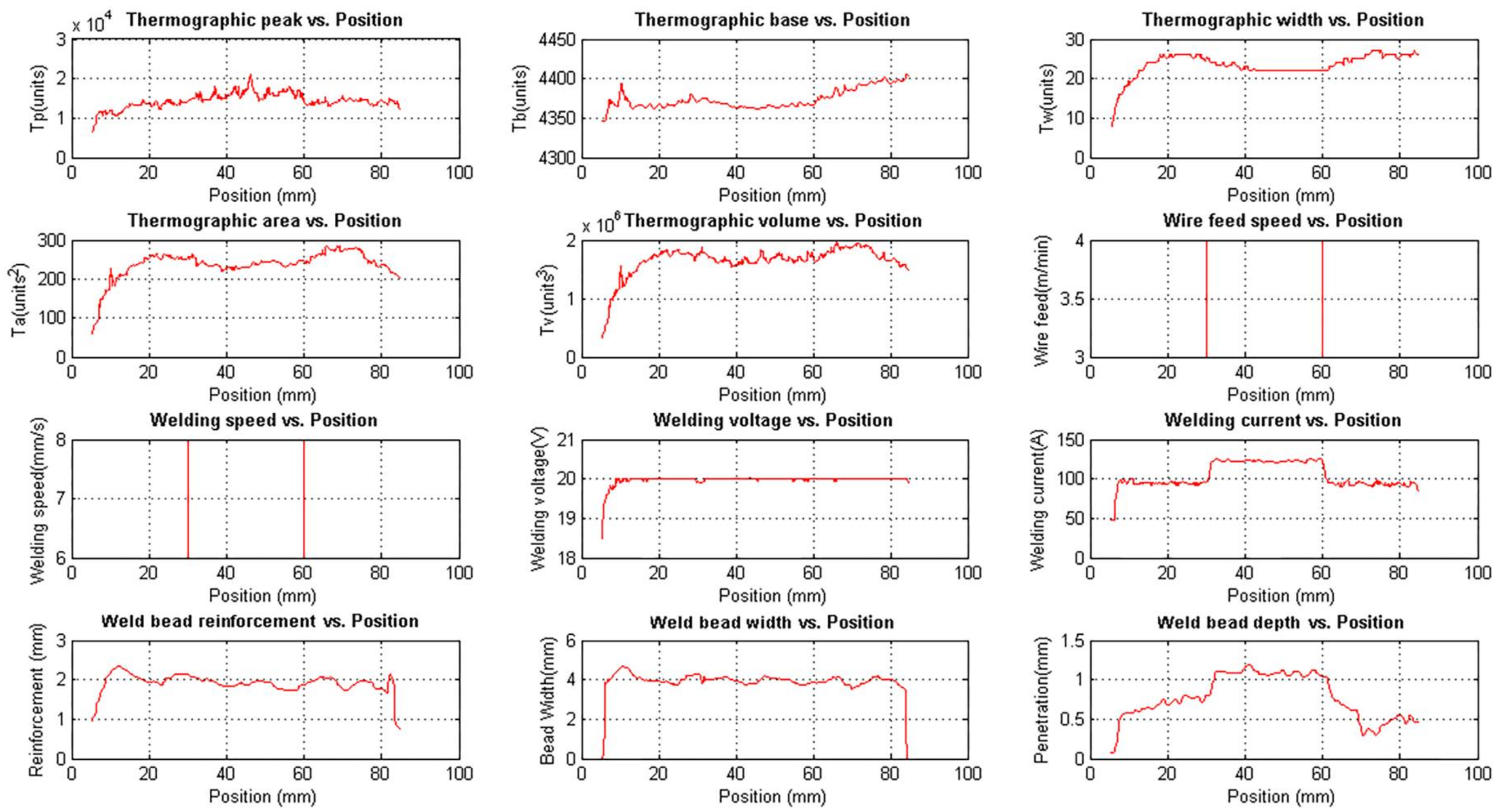
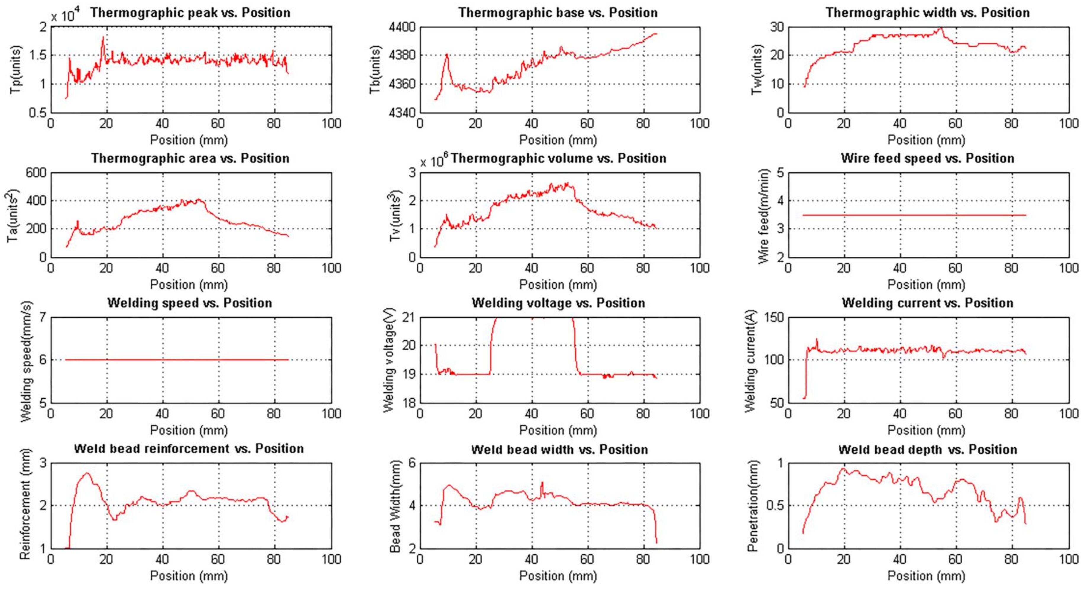
3.1.2. Experiment 2: Process Response to the Step in the Welding Voltage
3.2. Modelling and Validation of Estimators
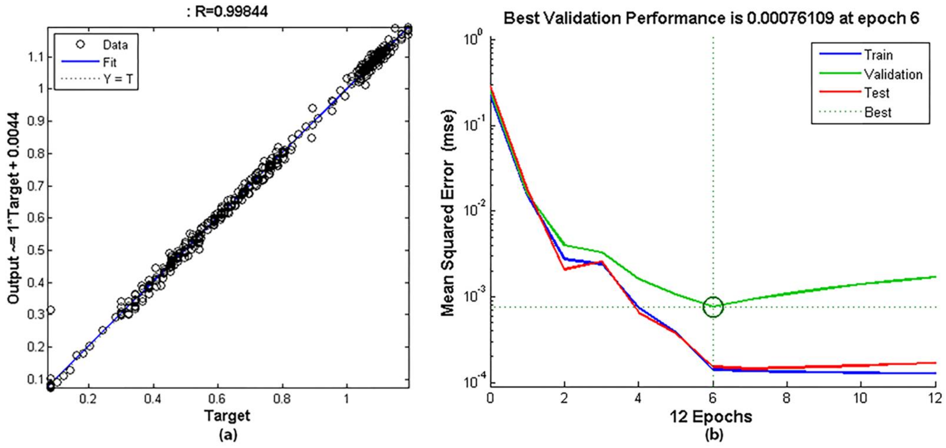
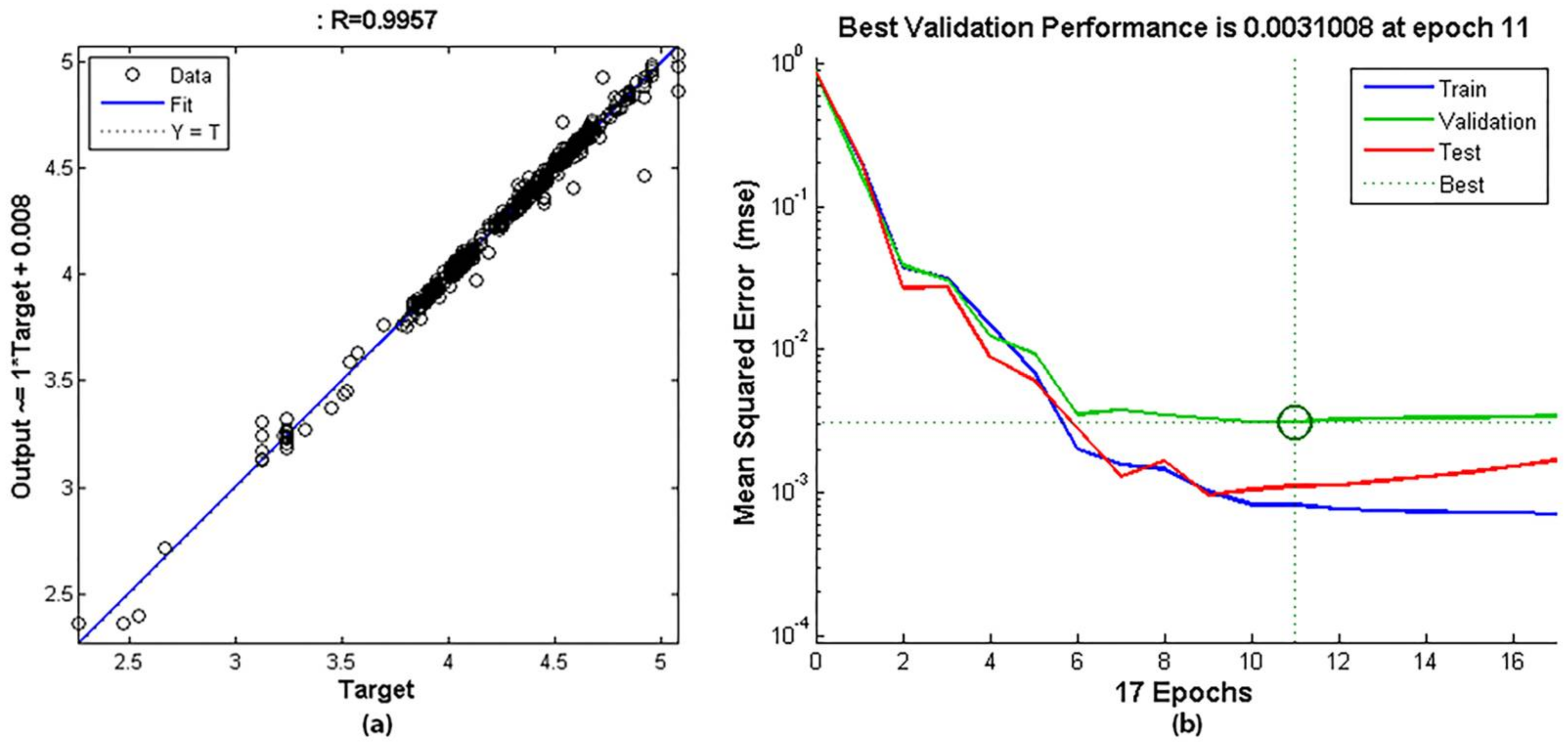
3.2.1. Training Results
3.2.2. Testing Results
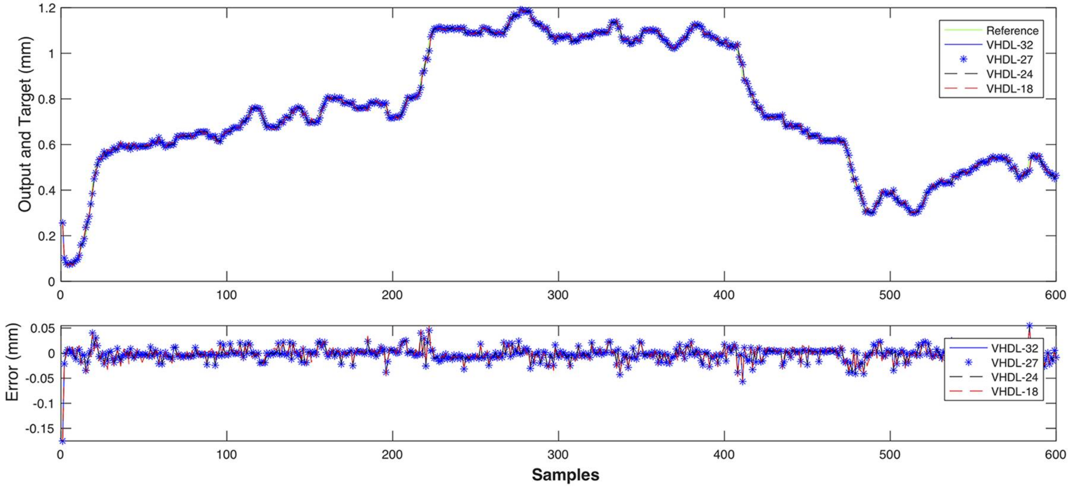
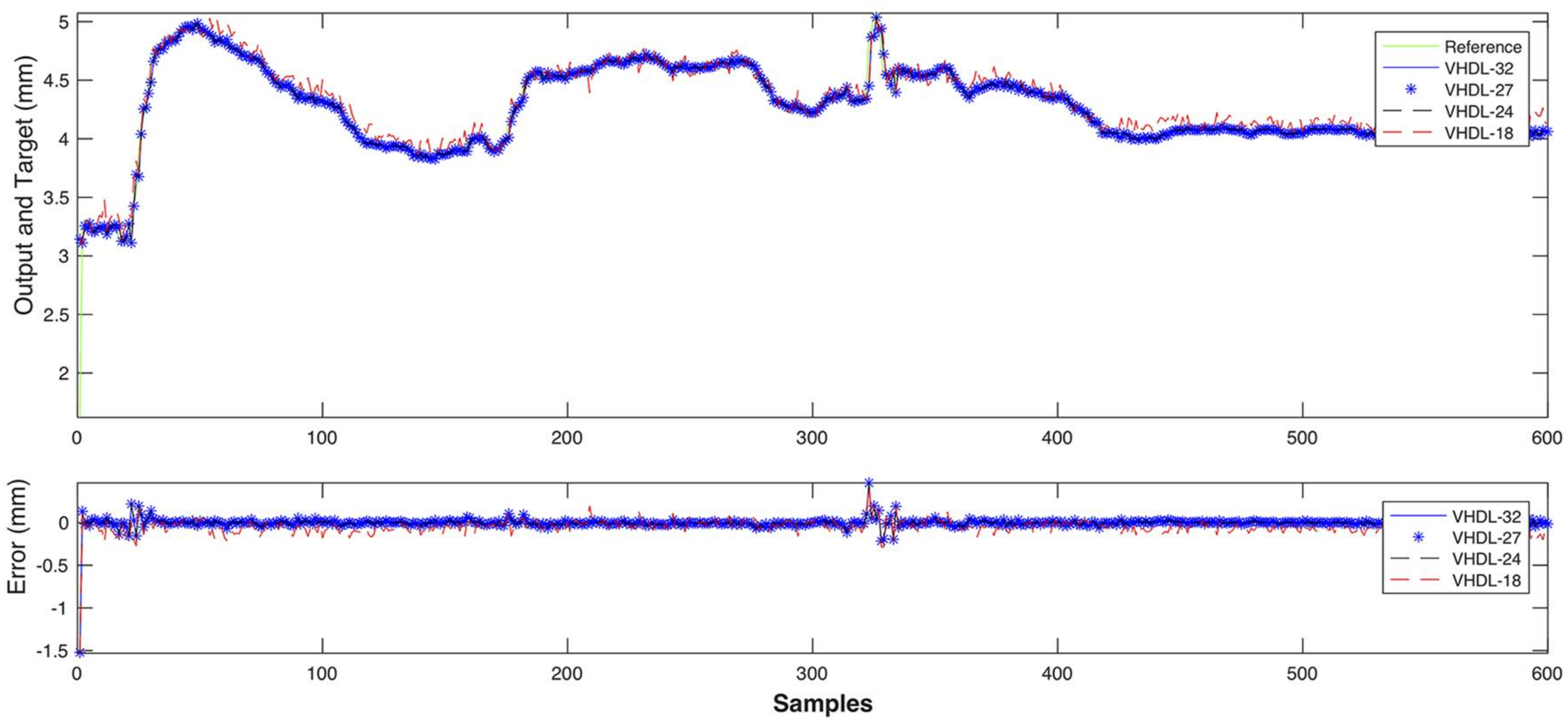
3.3. Simulations of Estimators in FPGA Device
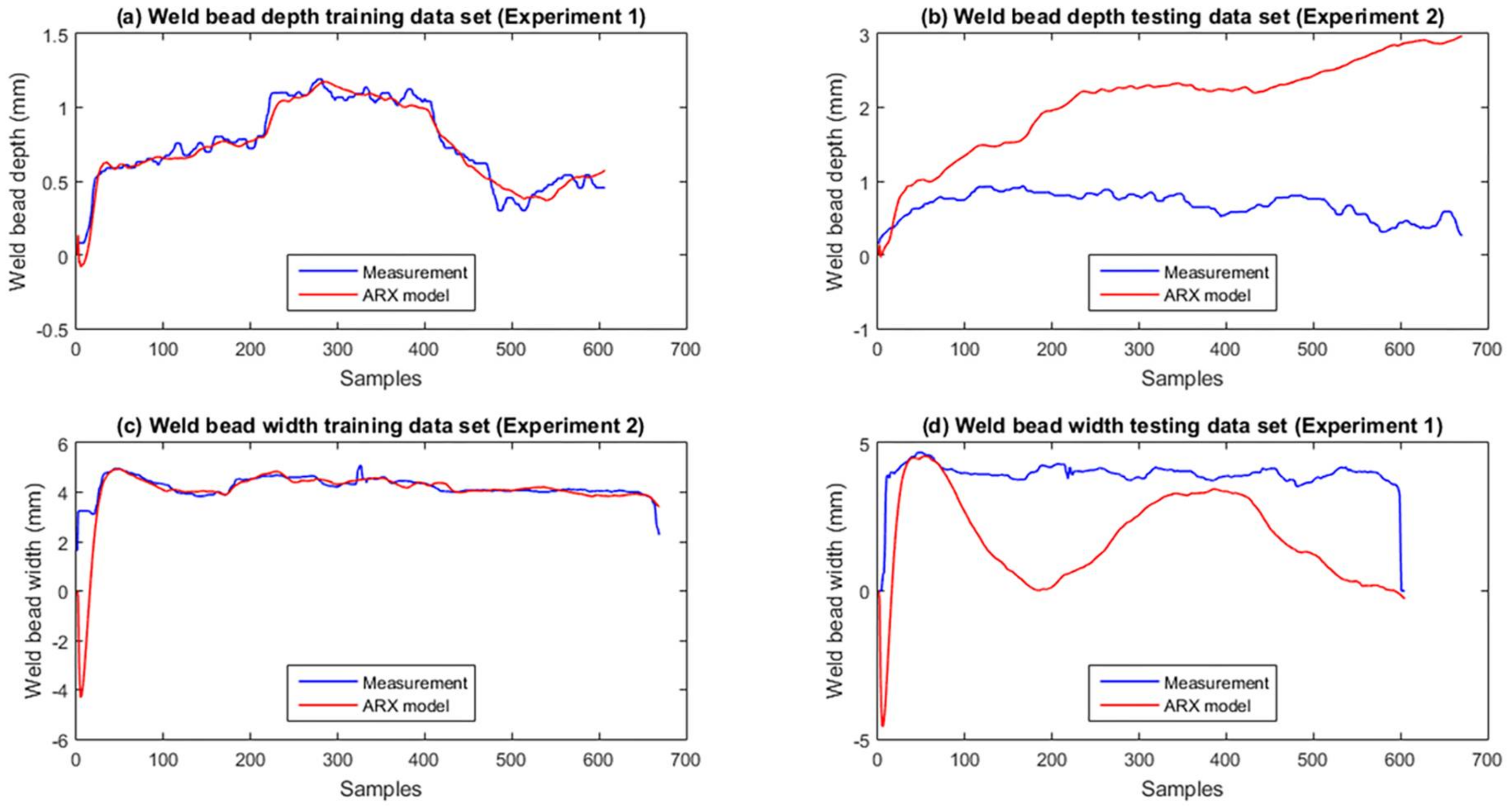
3.4. The Response of Autoregressive with Exogenous Inputs Linear Models
4. Conclusions
Acknowledgments
Author Contributions
Conflicts of Interest
References
- Bestard, G.A.; Alfaro, S.C.A. Propuesta de diseño de un sistema de control de la geometría del cordón en procesos de soldadura orbital. Rev. Control. Cibern. Autom. 2016, 4. [Google Scholar]
- American Welding Society Staff. Welding Science and Technology, 9th ed.; Jenney, C.L., O’Brien, A., Eds.; American Welding Society: Miami, FL, USA, 2002; Volume 1, ISBN 0-87171-657-7. [Google Scholar]
- Bestard, G.A. Sensor Fusion and Embedded Devices to Estimate and Control the Depth and Width of the Weld Bead in Real Time. Ph.D. Thesis, Universidade de Brasília, Brasília, Brazil, 2017. [Google Scholar]
- Brosed, F.J.; Aguilar, J.J.; Guillomïa, D.; Santolaria, J. 3D geometrical inspection of complex geometry parts using a novel laser triangulation sensor and a robot. Sensors 2011, 11, 90–110. [Google Scholar] [CrossRef] [PubMed]
- Luo, H.; Chen, X. Laser visual sensing for seam tracking in robotic arc welding of titanium alloys. Int. J. Adv. Manuf. Technol. 2005, 26, 1012–1017. [Google Scholar] [CrossRef]
- Liu, Y.; Zhang, W.; Zhang, Y. Estimation of Weld Joint Penetration under Varying GTA Pools. Weld. J. Suppl. AWS 2013, 92, 313–321. [Google Scholar]
- Liu, Y.; Zhang, Y. Control of 3D weld pool surface. Control Eng. Pract. 2013, 21, 1469–1480. [Google Scholar] [CrossRef]
- Liu, Y.K.; Zhang, W.J.; Zhang, Y.M. Nonlinear Modeling for 3D Weld Pool Characteristic Parameters in GTAW. Weld. J. 2015, 94, 231s–240s. [Google Scholar]
- Chen, W.H.; Nagarajan, S.; Chin, B.A. Weld penetration sensing and control. Infrared Technol. 1988, 972, 268–272. [Google Scholar]
- Nagarajan, S.; Chen, H.W.; Chin, B.A. Infrared sensing for adaptive arc welding. Weld. J. 1989, 68, 462–466. [Google Scholar]
- Nagarajan, S.; Banerjee, P.; Chen, W.; Chin, B.A. Weld pool size and position control using IR sensors. Proceedings of NSF Design and Manufacturing Systems Conference, Atlanta, GA, USA, 25–28 March 1990. [Google Scholar]
- Nagarajan, S.; Chin, B.A.; Chen, W. Control of the welding process using infrared sensors. IEEE Trans. Robot. Autom. 1992, 8, 86–93. [Google Scholar] [CrossRef]
- Beardsley, H.E.; Zhang, Y.M.M.; Kovacevic, R. Infrared sensing of full penetration state in gas tungsten arc welding. Int. J. Mach. Tool Manuf. 1994, 34, 1079–1090. [Google Scholar] [CrossRef]
- Chokkalingham, S.; Chandrasekhar, N.; Vasudevan, M. Predicting the depth of penetration and weld bead width from the infra red thermal image of the weld pool using artificial neural network modeling. J. Intell. Manuf. 2012, 23, 1995–2001. [Google Scholar] [CrossRef]
- Iceland, W.F.; Martin, E. O’Dor Weld Penetration Control. U.S. Patent 3567899A, 2 March 1971. [Google Scholar]
- Nomura, H.; Satoh, Y.; Tohno, K.; Satoh, Y.; Kuratori, M. Arc light intensity controls current in SA welding system. Weld. Met. Fabr. 1980, 90, 457–463. [Google Scholar]
- Bangs, E.R.; Longinow, N.E.; Blaha, J.R. Using Infrared Image to Monitor and Control Welding. U.S. Patent 4877940A, 30 October 1989. [Google Scholar]
- Bestard, G.A.; Alfaro, S.C.A. Sensor fusion: Theory review and applications. In Proceedings of the 23rd ABCM International Congress of Mechanical Engineering COBEM 2015, Rio de Janeiro, Brazil, 6–11 December 2015. [Google Scholar]
- Henderson, T.C.; Dekhil, M.; Kessler, R.R.; Griss, M.L. Sensor Fusion. Control Probl. Robot. Autom. 1998, 230, 193–207. [Google Scholar]
- Dong, J.; Zhuang, D.; Huang, Y.; Fu, J. Advances in Multi-Sensor Data Fusion: Algorithms and Applications. Sensors 2009, 9, 7771–7784. [Google Scholar] [CrossRef] [PubMed]
- Sasiadek, J.Z. Sensor fusion. Annu. Rev. Control 2002, 26, 203–228. [Google Scholar] [CrossRef]
- Song, J.B.; Hardt, D.E. Closed-loop control of weld pool depth using a thermally based depth estimate. Weld. J. 1993, 72, 471s–478s. [Google Scholar]
- Song, J.B.; Hardt, D.E. Multivariable adaptive control of bead geometry in GMA welding. Int. J. Press. Vessel. Pip. 2002, 79, 251–262. [Google Scholar]
- Chen, B.; Wang, J.; Chen, S. Modeling of pulsed GTAW based on multi-sensor fusion. Sens. Rev. 2009, 29, 223–232. [Google Scholar] [CrossRef]
- Chen, B.; Wang, J.; Chen, S. Prediction of pulsed GTAW penetration status based on BP neural network and D-S evidence theory information fusion. Int. J. Adv. Manuf. Technol. 2010, 48, 83–94. [Google Scholar] [CrossRef]
- Pal, K.; Pal, S.K. Monitoring of Weld Penetration Using Arc Acoustics. Mater. Manuf. Process. 2011, 26, 684–693. [Google Scholar] [CrossRef]
- Alfaro, S.C.A. Sensors for quality control in welding. Soldag. Insp. 2012, 17, 192–200. [Google Scholar] [CrossRef]
- Alfaro, S.C.A.; Cayo, E.H. Sensoring fusion data from the optic and acoustic emissions of electric arcs in the GMAW-S process for welding quality assessment. Sensors 2012, 12, 6953–6966. [Google Scholar] [CrossRef] [PubMed]
- Yu, H.; Ye, Z.; Chen, S. Application of arc plasma spectral information in the monitor of Al–Mg alloy pulsed GTAW penetration status based on fuzzy logic system. Int. J. Adv. Manuf. Technol. 2013, 68, 2713–2727. [Google Scholar] [CrossRef]
- Chen, B.; Chen, S.; Feng, J. A study of multisensor information fusion in welding process by using fuzzy integral method. Int. J. Adv. Manuf. Technol. 2014, 74, 413–422. [Google Scholar] [CrossRef]
- Liu, Y.; Zhang, Y. Fusing machine algorithm with welder intelligence for adaptive welding robots. J. Manuf. Process. 2017, 27, 18–25. [Google Scholar] [CrossRef]
- Dave, V.R.; Cola, M.J. Methods for Control of Fudion Welding Process by Maintaining a Controller Weld Pool Volume. U.S. Patent 8354608, 15 January 2013. [Google Scholar]
- Nefedyev, E.; Gomera, V.; Sudakov, A. Application of Acoustic Emission Method for Control of Manual Arc Welding, Submerged Arc Welding. In Proceedings of the 31st Conference of the European Working Group on Acoustic Emission (EWGAE), Dresden, Germany, 3–5 Septermber 2014; pp. 1–9. [Google Scholar]
- Yang, F.; Zhang, S.; Zhang, W.M. Design of GTAW Wire Feeder Control System Based on Nios II. Appl. Mech. Mater. 2013, 397–400, 1909–1912. [Google Scholar] [CrossRef]
- Hurtado, R.H.; Alfaro, S.C.A.; Llanos, C.H. Discontinuity welding detection using an embedded hardware system. ABCM Symp. Ser. Mechatron. 2012, 5, 879–888. [Google Scholar]
- Llanos, C.H.; Hurtado, R.H.; Alfaro, S.C.A. FPGA-based approach for change detection in GTAW welding process. J. Braz. Soc. Mech. Sci. Eng. 2016, 38, 913–929. [Google Scholar] [CrossRef]
- Velasco, R.H.H. Detecção on-line de Descontinuidades no Processo de Soldagem GTAW Usando Sensoriamento Infravermelho e FPGAs. Master’s Thesis, Universidade de Brasília, Brasília, Brazil, 2010. [Google Scholar]
- Machado, M.V.R.; Mota, C.P.; Neto, R.M.F.; Vilarinho, L.O. Sistema Embarcado para Monitoramento Sem Fio de Sinais em Soldagem a Arco Elétrico com Abordagem Tecnológica. Soldag. Insp. 2012, 17, 147–157. [Google Scholar] [CrossRef]
- Millán, R.; Quero, J.M.; Franquelo, L.G. Welding data adquisition based on FPGA. IC’s Instrum. Control 1997, 1, 2–6. [Google Scholar] [CrossRef]
- Bestard, G.A.; Alfaro, S.C.A. Sistema de adquisición de datos y control en lazo abierto para procesos de soldadura GMAW. In Proceedings of the Taller Internacional de Cibernética Aplicada TCA 2017, Vedado, Cuba, 21 February 2017; pp. 1–7. [Google Scholar]
- IMC-Soldagem Manual de Instruções Inversal 450/600. Available online: https://www.imc-soldagem.com.br/images/documentos/manuais/inversal_450-600_manual_instrucoes_2ed_(1998).pdf (accessed on 10 November 2017).
- Park, J.; Mackay, S.; Wright, E. Practical Data Communications for Instrumentation and Control; Elsevier: Amsterdam, The Netherlands, 2003; ISBN 07506 57979. [Google Scholar]
- Franco, F.D. Monitorização e localização de defeitos na soldagem TIG através do sensoriamento infravermelho. Master’s Thesis, Universidad de Brasília, Brasília, Brazil, 2008. [Google Scholar]
- Berger Lahr GmbH & Co. KG. Product Manual. Intelligent Compact Drive Pulse/Direction Stepper Motor IclA IDS; Berger Lahr GmbH & Co. KG: Lahr, Germany, 2006. [Google Scholar]
- Microchip Technology Inc. Pic18F4550. Available online: http://ww1.microchip.com/downloads/en/DeviceDoc/39632e.pdf (accessed on 10 November 2017).
- FLIR-Systems. ThermoVisionTM A40 M Manual del Usuario; FLIR-Systems: Wilsonville, OR, USA, 2004. [Google Scholar]
- Trade Association FireWire Design Guide. Available online: http://www.1394ta.org/developers/designguide/tafwdesignguide.pdf (accessed on 2 December 2017).
- FLIR-Systems ThermoVisionTM SDK User’s Manual. Available online: http://www.mds-flir.com/data/bbsData/ThermoVision SDK.pdf (accessed on 1 December 2017).
- MathWorks Hyperbolic Tangent Sigmoid Transfer Function—MATLAB Tansig. Available online: https://www.mathworks.com/help/nnet/ref/tansig.html (accessed on 19 July 2017).
- Ayala, H.V.H.; Muñoz, D.M.; Llanos, C.H.; dos Santos Coelho, L. Efficient hardware implementation of radial basis function neural network with customized-precision floating-point operations. Control Eng. Pract. 2017, 60, 124–132. [Google Scholar] [CrossRef]
- Ayala, H.; Sampaio, R.; Mu, D.M.; Llanos, C.; Coelho, L.; Jacobi, R. Nonlinear Model Predictive Control Hardware Implementation with Custom-precision Floating Point Operations. Proceedings of 24th Mediterranean Conference on Control and Automation (MED), 2016, Athens, Greece, 21–24 June 2016; IEEE, 2016. [Google Scholar] [CrossRef]
- Muñoz, D.M.; Sanchez, D.F.; Llanos, C.H.; Ayala-Rincón, M. Tradeoff of FPGA design of a floating-point library for arithmetic operators. J. Integr. Circuits Syst. 2010, 5, 42–52. [Google Scholar]
- Muñoz, D.M.; Sanchez, D.F.; Llanos, C.H.; Ayala-Rincón, M. FPGA based floating-point library for CORDIC algorithms. In Proceedings of the 2010 VI Southern Programmable Logic Conference (SPL), Ipojuca, Brazil, 24–26 March 2010; pp. 55–60. [Google Scholar]


| Position (mm) | Welding Speed (mm/s) | Welding Voltage (V) | Wire Feed Speed (m/min) | Arc Status |
|---|---|---|---|---|
| 5.0 | 6.0 | 20.0 | 3.0 | On |
| 30.0 | 8.0 | 20.0 | 4.0 | On |
| 60.0 | 6.0 | 20.0 | 3.0 | On |
| 85.0 | 6.0 | 20.0 | 3.0 | Off |
| Position (mm) | Welding Speed (mm/s) | Welding Voltage (V) | Wire Feed Speed (m/min) | Arc Status |
|---|---|---|---|---|
| 5.0 | 6.0 | 19.0 | 3.5 | On |
| 30.0 | 6.0 | 21.0 | 3.5 | On |
| 60.0 | 6.0 | 19.0 | 3.5 | On |
| 85.0 | 6.0 | 19.0 | 3.5 | Off |
| Estimator of | Weld Bead Depth | Weld Bead Width | ||
|---|---|---|---|---|
| Training (Exp. 1) | Test (Exp. 2) | Training (Exp. 2) | Test (Exp. 1) | |
| Fit (R) | 0.9984 | 0.9901 | 0.9957 | 0.8516 |
| Epoch | 6 | - | 11 | - |
| Open loop MSE | 7.6109 × 10⁻⁴ | 8.076 × 10⁻⁴ | 31.008 × 10⁻⁴ | 0.128 |
| Closed loop MSE | 6.4 × 10⁻³ | 0.224 | 0.094 | 0.67 |
| MPL Floating Point Precision | Weld Bead Depth Estimator MSE | Weld Bead width Estimator MSE |
|---|---|---|
| 32 bits | 2.095 × 10⁻⁴ | 5.045 × 10⁻³ |
| 27 bits | 2.095 × 10⁻⁴ | 5.046 × 10⁻³ |
| 24 bits | 2.094 × 10⁻⁴ | 5.056 × 10⁻³ |
| 18 bits | 2.460 × 10⁻⁴ | 1.186 × 10⁻² |
| Architecture Floating-Point Precision | ALMs Usage (Elements/%) | DSPs Usage (Elements/%) | Frequency (MHz) | Time (us) |
|---|---|---|---|---|
| 32 bits | 19,809/62% | 24/21% | 117.08 | 1.71 |
| 27 bits | 16,615/52% | 24/21% | 125.77 | 1.59 |
| 24 bits | 14,233/44% | 24/21% | 130.19 | 1.54 |
| 18 bits | 10,502/33% | 24/21% | 135.72 | 1.47 |
| Model Parameter | ARX Weld Bead Depth Model | ARX Weld Bead Width Model |
|---|---|---|
| Order of A (na) | 4 | 4 |
| Order of B+1 (nb) | [4 4 4 4 4 8] | [4 4 4 4 4 8] |
| Input-output delay (nk) | [1 1 1 1 1 1] | [1 1 1 1 1 1] |
| Fit Percent (Fit) | 79.87% | 59.09% |
| Mean squared error (MSE) in training | 0.0037 | 0.8029 |
| Mean squared error (MSE) in testing | 2.4464 | 6.4616 |
© 2018 by the authors. Licensee MDPI, Basel, Switzerland. This article is an open access article distributed under the terms and conditions of the Creative Commons Attribution (CC BY) license (http://creativecommons.org/licenses/by/4.0/).
Share and Cite
Bestard, G.A.; Sampaio, R.C.; Vargas, J.A.R.; Alfaro, S.C.A. Sensor Fusion to Estimate the Depth and Width of the Weld Bead in Real Time in GMAW Processes. Sensors 2018, 18, 962. https://doi.org/10.3390/s18040962
Bestard GA, Sampaio RC, Vargas JAR, Alfaro SCA. Sensor Fusion to Estimate the Depth and Width of the Weld Bead in Real Time in GMAW Processes. Sensors. 2018; 18(4):962. https://doi.org/10.3390/s18040962
Chicago/Turabian StyleBestard, Guillermo Alvarez, Renato Coral Sampaio, José A. R. Vargas, and Sadek C. Absi Alfaro. 2018. "Sensor Fusion to Estimate the Depth and Width of the Weld Bead in Real Time in GMAW Processes" Sensors 18, no. 4: 962. https://doi.org/10.3390/s18040962
APA StyleBestard, G. A., Sampaio, R. C., Vargas, J. A. R., & Alfaro, S. C. A. (2018). Sensor Fusion to Estimate the Depth and Width of the Weld Bead in Real Time in GMAW Processes. Sensors, 18(4), 962. https://doi.org/10.3390/s18040962