Sparse Reconstruction Based Robust Near-Field Source Localization Algorithm †


Abstract
:1. Introduction
2. α-Stable Distribution
3. Problem Formulation
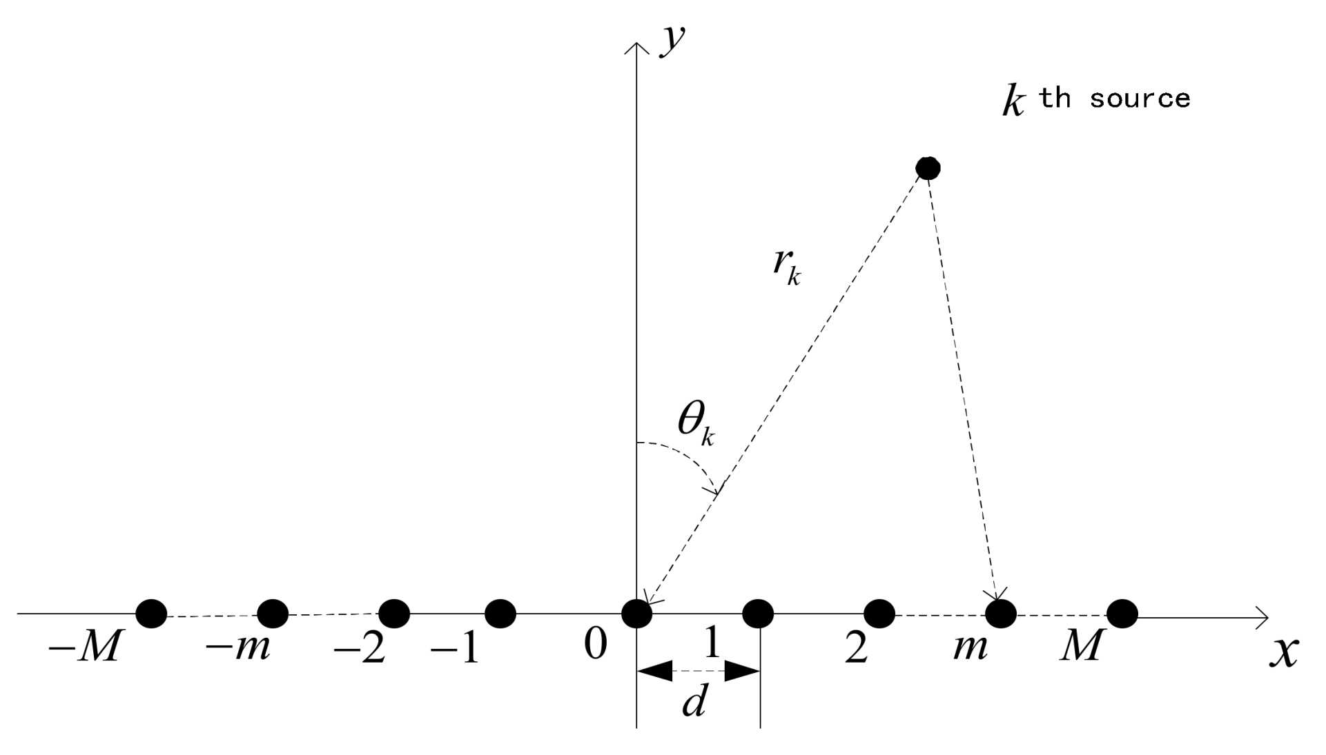
3.1. Signal Model
3.2. FLOC Matrix of the Array Received Signal
3.3. NTC Matrix of the Array Received Signal
4. Proposed Two Step Estimation Method
4.1. Step-1: DOA Estimation
4.2. Step-2: Range Estimation
5. Simulation Results
5.1. Simulation 1
5.2. Simulation 2
5.3. Simulation 3
5.4. Simulation 4
5.5. Simulation 5
5.6. Simulation 6
5.7. Simulation 7
6. Conclusions
Acknowledgments
Author Contributions
Conflicts of Interest
References
- Guo, R.; Zhang, Y.; Lin, Q.; Chen, Z. A Channelization-Based DOA Estimation Method for Wideband Signals. Sensors 2016, 16, 1031. [Google Scholar] [CrossRef] [PubMed]
- Krim, H.; Viberg, M. Two decades of array signal processing research: The parametric approach. IEEE Signal Process. Mag. 1996, 13, 67–94. [Google Scholar] [CrossRef]
- Tengtrairat, N.; Woo, W.L. Blind 3D sound source direction using stereo microphones based on time-delay estimation and polar-pattern histogram. In Proceedings of the 2nd International Conference on Information Technology, Bangkok, Thailand, 2–3 November 2017. [Google Scholar]
- Tengtrairat, N.; Parathai, P.; Woo, W.L. Blind 2D signal direction for limited-sensor space using maximum likelihood estimation. Asia Pac. J. Sci. Technol. 2017, 22, 42–49. [Google Scholar]
- Huang, Y.D.; Barkat, M. Near-field multiple sources localization by passive sensor array. IEEE Trans. Antennas Propag. 1991, 39, 968–975. [Google Scholar] [CrossRef]
- Starer, D.; Nehorai, A. Passive localization of near-field sources by path following. IEEE Trans. Signal Process. 1994, 42, 677–680. [Google Scholar] [CrossRef]
- Lee, J.H.; Lee, C.M.; Lee, K.K. A modified path-following algorithm using a known algebraic path. IEEE Trans. Signal Process. 1999, 47, 1407–1409. [Google Scholar]
- Zhi, W.; Chia, M.Y. Near-field source location via symmetric subarrays. IEEE Signal Process. Lett. 2007, 14, 409–412. [Google Scholar] [CrossRef]
- Liang, L.; Tao, J.W.; Huang, J.C. Near-field source location based on sparse symmetric array. Acta Electron. Sin. 2009, 37, 1307–1312. (In Chinese) [Google Scholar]
- Liu, H.B.; Chen, F.S. A near-field passive localization method. Infrared Laser Eng. 2007, 36, 610–613. (In Chinese) [Google Scholar]
- Liang, J.; Liu, D. Passive localization of mixed near-field and far-field sources using two-stage music algorithm. IEEE Trans. Signal Process. 2010, 58, 108–120. [Google Scholar] [CrossRef]
- Xie, J.; Tao, H.; Rao, X.; Su, J. Passive localization of mixed far-field and near-field sources without estimating the number of sources. Sensors 2015, 15, 3834–3853. [Google Scholar] [CrossRef] [PubMed]
- Challa, R.N.; Shamsunder, S. High-order subspace-based algorithms for passive localization of near-field sources. In Proceedings of the Twenty-Ninth Asilomar Conference on Signals, Systems and Computers, Pacific Grove, CA, USA, 30 October–2 November 1995; pp. 777–781. [Google Scholar]
- Liang, J.; Liu, D. Passive localization of near-field sources using cumulant. IEEE Sens. J. 2009, 9, 953–960. [Google Scholar] [CrossRef]
- Cekli, E.; Cirpan, H.A. Unconditional maximum likelihood approach for localization of near-field sources: Algorithm and performance analysis. AEU Int. J. Electron. Commun. 2003, 57, 9–15. [Google Scholar] [CrossRef]
- Grosicki, E.; Meraim, A.K.; Hua, Y. A weighted linear prediction method for near-field source localization. IEEE Trans. Signal Proc. 2005, 53, 3651–3660. [Google Scholar] [CrossRef]
- Hu, N.; Ye, Z.F.; Xu, X. DOA estimation for sparse array via sparse signal reconstruction. IEEE Trans. Aerosp. Electron. Syst. 2013, 49, 760–773. [Google Scholar] [CrossRef]
- Wang, B.; Liu, J.J.; Sun, X.Y. Mixed sources localization based on sparse signal reconstruction. IEEE Signal Process. Lett. 2012, 19, 487–490. [Google Scholar] [CrossRef]
- Tian, Y.; Sun, X.Y. Passive localization of mixed sources jointly using music and sparse signal reconstruction. AEU Int. J. Electron. Commun. 2014, 68, 534–539. [Google Scholar] [CrossRef]
- Lian, G.L.; Han, B.; Lin, W.S. Near-field sources localization based on sparse signal reconstruction. Chin. J. Electron. 2014, 42, 1041–1046. (In Chinese) [Google Scholar]
- Li, S.; Liu, W.; Zheng, D.; Hu, S.R.; He, W. Localization of near-field sources based on sparse signal reconstruction with regularization parameter selection. Int. J. Antennas Propag. 2017, 2017, 1260601. [Google Scholar] [CrossRef]
- Hu, K.; Chepuri, S.P.; Leus, G. Near-field source localization using sparse recovery techniques. In Proceedings of the International Conference on Signal Processing and Communications (SPCOM), Bangalore, India, 22–25 July 2014; pp. 1–5. [Google Scholar]
- Hu, K.; Chepuri, S.P.; Leus, G. Near-field source localization: Sparse recovery techniques and grid matching. In Proceedings of the IEEE 8th Sensor Array and Multichannel Signal Processing Workshop (SAM), Coruña, Spain, 22–25 June 2014; pp. 369–372. [Google Scholar]
- Zhang, Y.D.; Qin, S.; Amin, M.G. Near-field source localization based on sparse reconstruction of sensor-angle distribution. In Proceedings of the IEEE International Radar Conference, Arlington, VA, USA, 10–15 May 2015; pp. 10–15. [Google Scholar]
- Qin, S.; Zhang, Y.D.; Wu, Q.S.; Moeness, G.A. Structure-Aware Bayesian Compressive Sensing for Near-Field Source Localization Based on Sensor-Angle Distributions. Int. J. Antennas Propag. 2015, 2015, 783467. [Google Scholar] [CrossRef]
- Button, M.D.; Gardiner, J.G.; Glover, I.A. Measurement of the impulsive noise environment for satellite-mobile radio systems at 1.5 GHz. IEEE Trans. Veh. Technol. 2002, 51, 551–560. [Google Scholar] [CrossRef]
- Nikias, C.L.; Shao, M. Signal Processing with Alpha-Stable Distributions and Applications; Wiely: New York, NY, USA, 1995. [Google Scholar]
- Li, S.; He, R.X.; Lin, B.; Sun, F. DOA Estimation Based on Sparse Representation of the Fractional Lower Order Statisticsin Impulsive Noise. IEEE/CAA J. Autom. Sin. 2016, 1–9. [Google Scholar] [CrossRef]
- Belkacemi, H.; Marcos, S. Robust subspace-based algorithms for joint angle/Doppler estimation in non-Gaussian clutter. Signal Process. 2007, 87, 1547–1558. [Google Scholar] [CrossRef]
- Ma, J.Q.; Ge, L.D.; Tong, L. A new DOA algorithm based on nonlinear compress core Function in symmetric α-stable distribution noise environment. Telecommun. Eng. 2014, 54, 34–39. [Google Scholar]
- Ma, J.Q.; Ge, L.D.; Tong, L. A TDE method based on nonlinear compress core function for HF fading signal in impulsive noise. In Proceedings of the 8th International Conference on Broadband Communications & Biomedical Applications, Guilin, China, 12–15 December 2013; pp. 108–113. [Google Scholar]
- Wang, B.; Wang, S.X. A method for two dimensional parameters estimation of near-field sources in impulsive noise environments. J. Circuits Syst. 2005, 10, 5–9. (In Chinese) [Google Scholar]
- Qiu, T.S.; Wang, P. A Novel Method for Near-Field Source Localization in Impulsive Noise Environments. Circuits Syst. Signal Process. 2016, 35, 4030–4059. [Google Scholar] [CrossRef]
- Li, S.; Lin, B.; Li, B.; He, R.X. Near-Field Localization Algorithm Based on Sparse Reconstruction of the Fractional Lower Order Correlation Vector. In Proceedings of the International Conference on Wireless Algorithms, Systems, and Applications, Guilin, China, 19–21 June 2017; pp. 903–908. [Google Scholar]
- Grant, M.; Boyd, S.; Ye, Y. CVX: Matlab Software for Disciplined Convex Programming, CVX Research, Inc.: Austion, TX, USA, 2008.


© 2018 by the authors. Licensee MDPI, Basel, Switzerland. This article is an open access article distributed under the terms and conditions of the Creative Commons Attribution (CC BY) license (http://creativecommons.org/licenses/by/4.0/).
Share and Cite
Li, S.; Li, B.; Lin, B.; Tang, X.; He, R. Sparse Reconstruction Based Robust Near-Field Source Localization Algorithm. Sensors 2018, 18, 1066. https://doi.org/10.3390/s18041066
Li S, Li B, Lin B, Tang X, He R. Sparse Reconstruction Based Robust Near-Field Source Localization Algorithm. Sensors. 2018; 18(4):1066. https://doi.org/10.3390/s18041066
Chicago/Turabian StyleLi, Sen, Bing Li, Bin Lin, Xiaofang Tang, and Rongxi He. 2018. "Sparse Reconstruction Based Robust Near-Field Source Localization Algorithm" Sensors 18, no. 4: 1066. https://doi.org/10.3390/s18041066
APA StyleLi, S., Li, B., Lin, B., Tang, X., & He, R. (2018). Sparse Reconstruction Based Robust Near-Field Source Localization Algorithm. Sensors, 18(4), 1066. https://doi.org/10.3390/s18041066